Chebyshev polynomials are a sequence of orthogonal polynomials that play a central role in numerical analysis, approximation theory, and applied mathematics. They are named after the Russian mathematician Pafnuty Chebyshev and come in two primary types: Chebyshev polynomials of the first kind (\(T_n(x)\)) and Chebyshev polynomials of the second kind (\(U_n(x)\)). In this post we are going to focus on the Chebyshev polynomials of the first kind.
Chebyshev Polynomials of the First Kind
There are many different ways to define the Chebyshev polynomials of the first kind. The one that seems most logical to me and most useful in terms of outlining various properties of the polynomials is
Looking at \eqref{eq:1} it is not obvious why \(T_{n}(x)\) would be a polynomial. In order to show it is indeed a polynomial let's recall the de Moivre's formula
We can apply binomial expansion and take the real part from it to obatin
where
denotes the binomal coefficient. We can also notice that
showing that \eqref{eq:2} is a polynomial of \(\cos{\theta}\) of degree \(n\). Now, let
and by utilising \(\cos{\left(\arccos{x}\right)} = x\) we get
This transforms \eqref{eq:1} to
which we already showed is a polynomial of degree \(n\). From here, because \(\cos(.)\) is an even function, we can note that
From \eqref{eq:3} it is also obvious that the values of \(T_n\) in the interval \([-1, 1]\) are bounded in \([-1, 1]\) because of the cosine.
Chebyshev Nodes of the First Kind
Before we continue with exploring the roots of the polynomials, let's recall some trigonometry.
The unit circle is a circle with a radius of 1, centered at the origin of the Cartesian coordinate system. Below is shown part of the unit circle corresponding to the region from \(0\) to \(\frac{\pi}{2}\).

The cosine of an angle \(\theta\) corresponds to the \(x\)-coordinate of the point where the terminal side of the angle (measured counterclockwise from the positive \(x\)-axis) intersects the unit circle. In other words, \(\cos(\theta)\) gives the horizontal distance from the origin to this intersection point.
The arccosine is the inverse function of cosine, and it maps a cosine value back to its corresponding angle in the range \([0, \pi]\) radians. For a given \(x\)-coordinate on the unit circle, the arccosine gives the angle \(\theta\) such that \(\cos(\theta) = x\), meaning
Moreover, a radian is defined as the angle subtended at the center of a circle by an arc whose length is equal to the radius of the circle. For any circle, the length of an arc \(s\) is given by
where \(r\) is the radius of the circle, \(\theta\) is the angle subtended by the arc at the center. This means that on the unit circle the length of the arc equals the measure of the angle in radians because \(r = 1\), and hence
Now, let's find the roots of the polynomial \(T_{n}(x)\). If we take the definition in \eqref{eq:1} we have to solve
The solutions in the interval \((-1, 1)\) are given by
These roots are known as the Chebyshev nodes of the first kind, or the Chebyshev zeros. If we are working with an arbitrary interval \((a, b)\) the affine transformation
is needed. From the cosine properties we can also note that the nodes are symmetric with respect to the midpoint of the interval, and that the extrema of \(T_n(x)\) over the interval \([-1, 1]\) alternate between \(-1\) and \(1\). Also, a very useful fact is that these nodes are used in polynomial interpolation to minimize the Runge phenomenon.
In the figure below we have shown the roots of \(T_{8}(x)\) in blue. We have also built the perpendiculars from the roots to their interesction with the upper half of the unit circle, and marked these points in red.

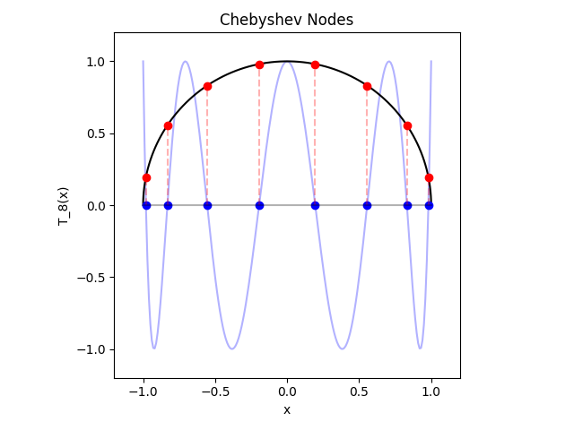
Looking at the figure we can notice that the arc lengths between the red points seem to be of the same length. Let's show that this is indeed the truth.
We showed the roots are the cosine functions \(\cos{\left(\frac{2k - 1}{2n}\pi\right)}, n \in N, k = 1, 2, ...n\). Thus, in the unit circle we have that the length of the corresponding arcs are equal to \(\left( \frac{2k - 1}{2n}\pi \right), n \in N, k = 1, 2, ...n\). Let's take two red points which are direct neighbours, or in other words let's take two red points corresponding to the randomly chosen \(m\) and \(m + 1\) roots, \(m \in k = \{1, 2, ..., n\}\). If we subtract them we are going to determine the length of the arc between them. We have
meaning that between every two nodes the arc length is equal and has a value of \(\frac{\pi}{n}\). A polynomial of degree \(n\) has \(n\) roots, which in our case are in the open interval \((-1, 1)\), meaning the arcs corresponding to every two neighbouring roots are \(n - 1\), and the two arcs between the \(x\)-axis and the first and last roots due to the symmetry of roots have lenghts of
Recurrence relation
This is probably a bit out of nowhere, but let's take a look at the following trigonometric identity
and show that the left side indeed is equal to the right one. We are going to need the following two fundamental formulas of angle addition in trigonometry
and
In our case we have
and
Adding the above equations leads to the wanted result.
Now, we can see that the terms of \eqref{eq:4} are exactly in the form of the right side of \eqref{eq:1}, \eqref{eq:3}, hence we get
or we get the useful recurrence relation
This relation along with adding \(T_{0}(x) = 1\) and \(T_{1}(x) = x\) is another famous way to define the Chebyshev polynomials of the first kind, or
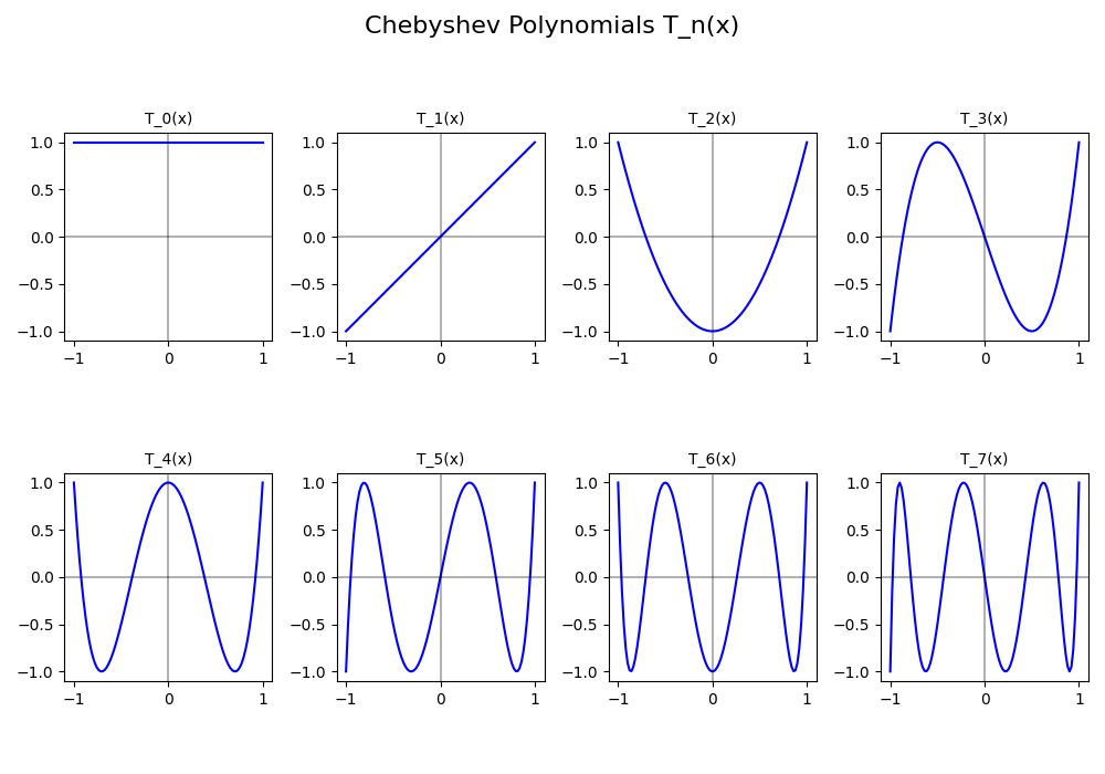
Let's write the first \(6\) polynomials by using \eqref{eq:6}:
We can notice that
and \(T_{k}(x)\) is alternating between an even and an odd polynomial depending on whether \(k\) is even or odd respectively.
Before we continue with some visualisations and more facts, let's mention that an interesting way to represent the recurrence relation \eqref{eq:5} is via the determinant
Now, let's visualise the first \(8\) polynomials.
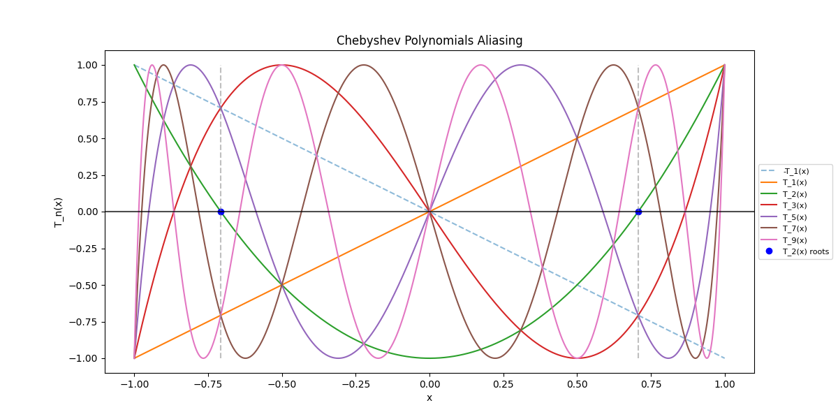
But what can we notice if we stack them together?
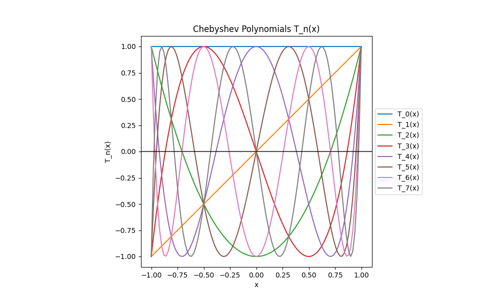
It is quite obvious that at the roots of the \(N\)-th Chebyshev polynomial there is an aliasing effect, meaning higher order polynomials look like lower order ones. We can formally show it by fixing \(N\), at the roots \(x_k\) of \(T_{N}(x) = 0\), and using the Chebyshev identity
or equivalently
Now, having \(T_{N}(x) = 0\) leads to
If we consecutevly set \(m = N\), \(m = 2N\), ..., \(m = 6N\), etc. we would get
We can safely say that any higher-order Chebyshev polynomial \(T_{N}(x)\) can be reduced to a lower-order \(j, 0 \leq j \leq N\) Chebyshev polynomial at the sample points \(x_k\) which are the roots of \(T_{N}(x)\). In the figure below we attempt to visualise this statement.

The horizontal axis represents the order of Chebyshev polynomials, and the blue wavy line represents a "folded ribbon". Think of it as taking the sequence of polynomial orders and folding it back and forth. This folding happens at specific points where higher-order polynomials can be reduced to lower-order ones, which are the red x marks showing the sample points: the roots of \(T_n(x)\). The key insight is that at these special sample points, we don't need to work with the higher-order polynomials because we can use equivalent lower-order ones instead. This is incredibly useful in numerical computations as it can help reduce computational complexity, and makes the Chebyshev polynomials very computationally efficient.
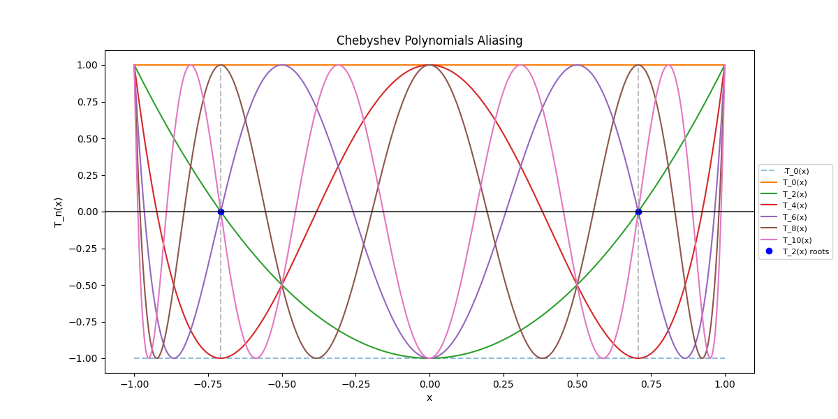
Let's illustarte this with a simple example. Let \(N = 2\), then for even \(m\) we have
In the figure below we can see the even polynomials and that indeed \(T_{10}(x)\) behaves like \(-T_{6}(x)\) which behaves like \(T_{2}(x)\) at the roots having value \(0\), \(T_{8}(x)\) behaves like \(-T_{4}(x)\) at the roots with value \(1\) as in \(T_{0}(x)\), \(T_{6}(x)\) behaves like \(-T_{2}(x)\) with value \(0\), and \(T_{4}(x)\) behaves like \(-T_{0}(x)\) with value \(-1\).
Click to expand code
from typing import Union

import matplotlib.pyplot as plt
import numpy as np


def chebyshev_polynomial(
    n: int, x: Union[float, np.ndarray]
) -> Union[float, np.ndarray]:
    """
    Calculate nth Chebyshev polynomial of the first kind T_n(x).

    Args:
        n: Order of polynomial (non-negative integer)
        x: Point(s) at which to evaluate polynomial

    Returns:
        Value of T_n(x)
    """
    if n < 0:
        raise ValueError("Order must be non-negative")

    if n == 0:
        return np.ones_like(x)
    elif n == 1:
        return x
    else:
        t_prev = np.ones_like(x)  # T_0
        t_curr = x  # T_1

        for _ in range(2, n + 1):
            t_next = 2 * x * t_curr - t_prev
            t_prev = t_curr
            t_curr = t_next

        return t_curr


def chebyshev_nodes(n):
    """Generate n Chebyshev nodes in [-1,1]"""
    k = np.arange(1, n + 1)
    return np.cos((2 * k - 1) * np.pi / (2 * n))


if __name__ == "__main__":

    x = np.linspace(-1, 1, 1000)
    plt.figure(figsize=(12, 6))
    plt.plot(x, -chebyshev_polynomial(0, x), "--", label=f"-T_{0}(x)", alpha=0.5)
    for n in [0, 2, 4, 6, 8, 10]:
        y = chebyshev_polynomial(n, x)
        plt.plot(x, y, label=f"T_{n}(x)")

    # plot nodes for n = 2
    n = 2
    nodes = chebyshev_nodes(n)
    y_nodes = np.cos(n * np.arccos(nodes))
    plt.plot(nodes, np.zeros_like(nodes), "bo", label="T_2(x) roots")
    for node in nodes:
        plt.plot([node, node], [-1, 1], "--", color="gray", alpha=0.5)

    # plt.grid(True)
    # Set aspect ratio to be equal
    # plt.gca().set_aspect('equal', adjustable='box')
    plt.xlabel("x")
    plt.ylabel("T_n(x)")
    plt.title("Chebyshev Polynomials Aliasing")
    plt.legend(loc="center left", bbox_to_anchor=(1, 0.5), fontsize=8)
    plt.xlim(-1.1, 1.1)
    plt.ylim(-1.1, 1.1)
    plt.axhline(y=0, color="k", linestyle="-", alpha=0.7)
    plt.savefig(
        "content/images/2025-01-06-chebyshev-polynomials/chebyshev_polynomials_aliasing_even.png"
    )
    plt.show()
For odd \(m\) we have
In the figure below we can see the odd polynomials and the aliasing as in the previous example.
Click to expand code
from typing import Union

import matplotlib.pyplot as plt
import numpy as np


def chebyshev_polynomial(
    n: int, x: Union[float, np.ndarray]
) -> Union[float, np.ndarray]:
    """
    Calculate nth Chebyshev polynomial of the first kind T_n(x).

    Args:
        n: Order of polynomial (non-negative integer)
        x: Point(s) at which to evaluate polynomial

    Returns:
        Value of T_n(x)
    """
    if n < 0:
        raise ValueError("Order must be non-negative")

    if n == 0:
        return np.ones_like(x)
    elif n == 1:
        return x
    else:
        t_prev = np.ones_like(x)  # T_0
        t_curr = x  # T_1

        for _ in range(2, n + 1):
            t_next = 2 * x * t_curr - t_prev
            t_prev = t_curr
            t_curr = t_next

        return t_curr


def chebyshev_nodes(n):
    """Generate n Chebyshev nodes in [-1,1]"""
    k = np.arange(1, n + 1)
    return np.cos((2 * k - 1) * np.pi / (2 * n))


if __name__ == "__main__":

    x = np.linspace(-1, 1, 1000)
    plt.figure(figsize=(12, 6))
    plt.plot(x, -chebyshev_polynomial(1, x), "--", label=f"-T_{1}(x)", alpha=0.5)
    for n in [1, 2, 3, 5, 7, 9]:
        y = chebyshev_polynomial(n, x)
        plt.plot(x, y, label=f"T_{n}(x)")

    # plot nodes for n = 2
    n = 2
    nodes = chebyshev_nodes(n)
    y_nodes = np.cos(n * np.arccos(nodes))
    plt.plot(nodes, np.zeros_like(nodes), "bo", label="T_2(x) roots")
    for node in nodes:
        plt.plot([node, node], [-1, 1], "--", color="gray", alpha=0.5)

    # plt.grid(True)
    # Set aspect ratio to be equal
    # plt.gca().set_aspect('equal', adjustable='box')
    plt.xlabel("x")
    plt.ylabel("T_n(x)")
    plt.title("Chebyshev Polynomials Aliasing")
    plt.legend(loc="center left", bbox_to_anchor=(1, 0.5), fontsize=8)
    plt.xlim(-1.1, 1.1)
    plt.ylim(-1.1, 1.1)
    plt.axhline(y=0, color="k", linestyle="-", alpha=0.7)
    plt.savefig(
        "content/images/2025-01-06-chebyshev-polynomials/chebyshev_polynomials_aliasing_odd.png"
    )
    plt.show()
Radial Plots
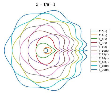
An interesting plot can be observed by plotting \(T_n(x)\) radially. This means that instead of evaluating the polynomials over \([-1, 1]\) in a Cartesian plane we are evaluating them at \(\frac{\theta}{\pi} - 1\), and plotting \(r = n + T_n(\frac{\theta}{\pi} - 1)\) on polar axes. In other words, the input domain has been shifted and extended, and the results are drawn as radial distances \(r\) around a circle defined by \(\theta\). This creates a polar visualization where each \(n\) produces a distinct spiral-like ornament. We are also filling in the areas between the curves for a visual effect.
Click to expand code
import matplotlib.pyplot as plt
import numpy as np
from numpy.polynomial.chebyshev import Chebyshev

theta = np.linspace(0, 2 * np.pi, 2000)
fig, ax = plt.subplots(subplot_kw={"projection": "polar"})

# Generate and fill between consecutive curves
for n in range(0, 19 * 2, 2):
    r1 = n + Chebyshev([0] * n + [1])(theta / np.pi - 1)
    r2 = (n + 2) + Chebyshev([0] * (n + 2) + [1])(theta / np.pi - 1)

    # Create black and white alternating pattern
    if n % 4 == 0:
        ax.fill_between(theta, r1, r2, color="black")
    else:
        ax.fill_between(theta, r1, r2, color="white")
ax.set_title("x = t/π - 1", y=1)
plt.axis("off")
plt.show()
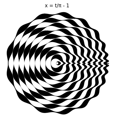
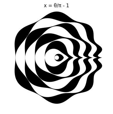
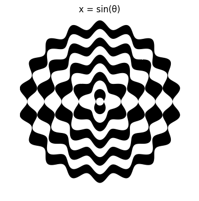
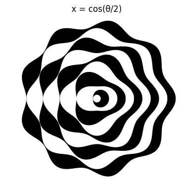
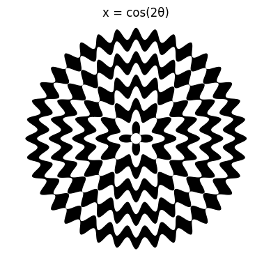
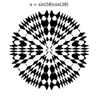
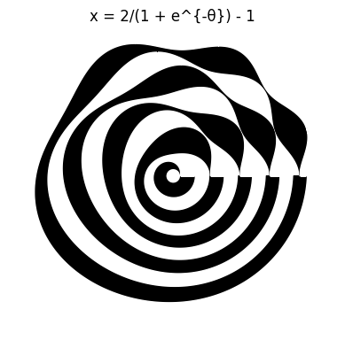
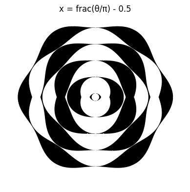
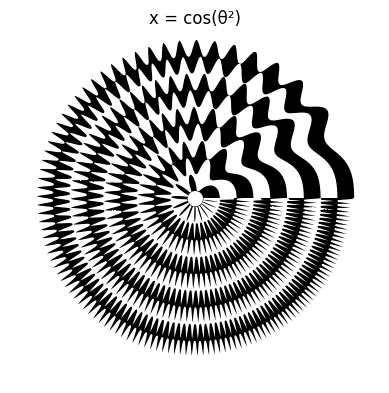
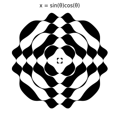
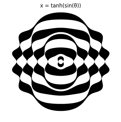
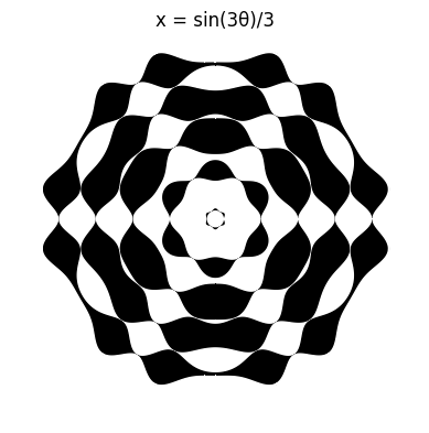
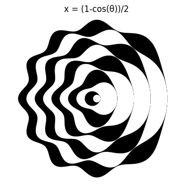
More visualusations can be achieved by doing other domain changes. They can be seen below.
In a separate post, Chebyshev Polynomials, Part 2, we are going to explore the Chebyshev polynomials of the second kind, and their relations to the polynomials of the first kind.