Partial differential equations...
Introduction
Let \(u(x, y, t)\) be ...
The homogenous wave equation is given by
or
Physical interpretation
The wave equation is a simplified model for a vibrating string (𝑛 = 1), membrane (𝑛 = 2), or elastic solid (𝑛 = 3). In these physical interpretations 𝑢(𝑥, 𝑡) represents the displacement in some direction of the point 𝑥 at time 𝑡 ≥ 0.
1D and 2D Equations
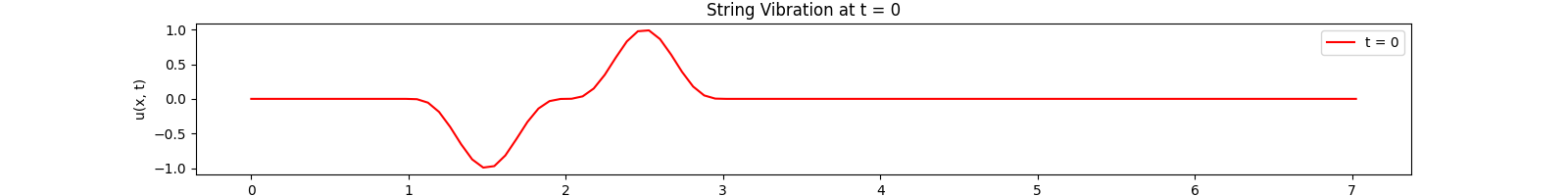
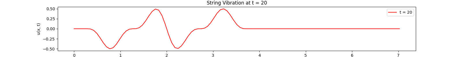
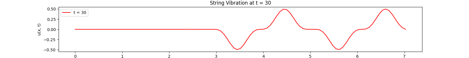
Fixed String
...
and
for \(t \in [0, 30]\). Using the \(100\)-th partial Fourier sum, \(L = \pi \sqrt{5}\), \(a = \frac{2}{3}\)...
Animation:
Click to expand code
import matplotlib.pyplot as plt
import numpy as np
from matplotlib.animation import FuncAnimation

# Define constants
L = np.pi * np.sqrt(5)
a = 2 / 3
tmax = 30
x = np.linspace(0, L, 101)
t = np.linspace(0, tmax, 200)


# Define the initial condition phi(x)
def phi(x):
    y = np.zeros_like(x)
    y[(1 < x) & (x < 3)] = np.sin(np.pi * x[(1 < x) & (x < 3)]) ** 3
    return y


# Define the initial velocity psi(x)
def psi(x):
    return np.zeros_like(x)


# Define the Fourier solution for u(x, t)
def fourier_u(x, t):
    y = np.zeros_like(x)
    for k in range(1, 101):
        Xk = np.sin(k * np.pi * x / L)
        Ak = (2 / L) * np.trapezoid(phi(x) * Xk, x)
        Bk = (2 / (a * k * np.pi)) * np.trapezoid(psi(x) * Xk, x)
        Tk = Ak * np.cos(a * k * np.pi * t / L) + Bk * np.sin(a * k * np.pi * t / L)
        y += Tk * Xk
    return y


# Set up the figure for animation
fig, ax = plt.subplots(figsize=(16, 2))
ax.set_xlim(0, L)
ax.set_ylim(-1, 1)
ax.set_xlabel("x")
ax.set_ylabel("u(x, t)")
ax.set_title("String Vibration")
(line,) = ax.plot([], [], lw=2, color="r")
(marker_left,) = ax.plot([], [], "ko", markerfacecolor="k")
(marker_right,) = ax.plot([], [], "ko", markerfacecolor="k")


def init():
    line.set_data([], [])
    marker_left.set_data([], [])
    marker_right.set_data([], [])
    return line, marker_left, marker_right


def update(frame):
    y = fourier_u(x, frame)
    line.set_data(x, y)
    marker_left.set_data([0], [y[0]])
    marker_right.set_data([L], [y[-1]])
    return line, marker_left, marker_right


# Create the animation
anim = FuncAnimation(fig, update, frames=len(t), init_func=init, blit=True)
anim.save("string_vibration_animation.gif", writer="pillow", fps=20)

plt.show()
Snapshots:
Rectangular Membrane
Pass
...
...
and ...
Solution... :
where
From the initial conditions it follows
and
Example 1
...
Solution:
where
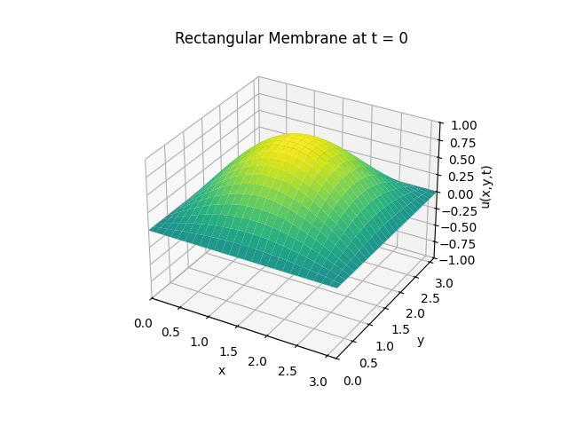
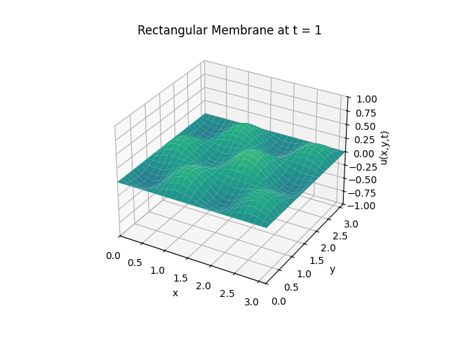
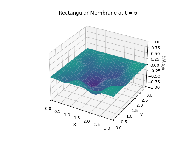
Therefore, \(A_{1, 1} = 1\), \(B_{4, 3} = \frac{1}{5}\), and every other coefficients is equal to \(0\). Finally,
For \(t \in [0, 6]\):
Animation:
Click to expand code
import matplotlib.pyplot as plt
import numpy as np
from matplotlib.animation import FuncAnimation


def rectangular_membrane_1(t_max: int = 6):
    t = np.linspace(0, t_max, 100)  # Time points for animation
    x = np.linspace(0, np.pi, 51)  # x grid
    y = np.linspace(0, np.pi, 51)  # y grid
    X, Y = np.meshgrid(x, y)

    # Define the solution function
    def solution(x, y, t):
        return (
            np.cos(np.sqrt(2) * t) * np.sin(x) * np.sin(y)
            + np.sin(5 * t) * np.sin(4 * x) * np.sin(3 * y) / 5
        )

    # Set up the figure and axis for animation
    fig = plt.figure()
    ax = fig.add_subplot(111, projection="3d")
    ax.set_xlim(0, np.pi)
    ax.set_ylim(0, np.pi)
    ax.set_zlim(-1, 1)
    ax.set_xlabel("x")
    ax.set_ylabel("y")
    ax.set_zlabel("u(x,y,t)")
    ax.set_title("Rectangular Membrane")

    # Update function for FuncAnimation
    def update(frame):
        ax.clear()  # Clear the previous frame
        Z = solution(X, Y, frame)  # Compute the new Z values
        _ = ax.plot_surface(X, Y, Z, cmap="viridis", vmin=-1, vmax=1)
        ax.set_xlim(0, np.pi)
        ax.set_ylim(0, np.pi)
        ax.set_zlim(-1, 1)
        ax.set_xlabel("x")
        ax.set_ylabel("y")
        ax.set_zlabel("u(x,y,t)")
        ax.set_title("Rectangular Membrane")

    # Create and save the animation
    anim = FuncAnimation(fig, update, frames=t, interval=50)
    anim.save("rectangular_membrane_1_animation.gif", writer="imagemagick", fps=20)

    plt.show()
Snapshots:
Example 2
...
Solution with Fourier method:
where
and
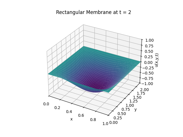
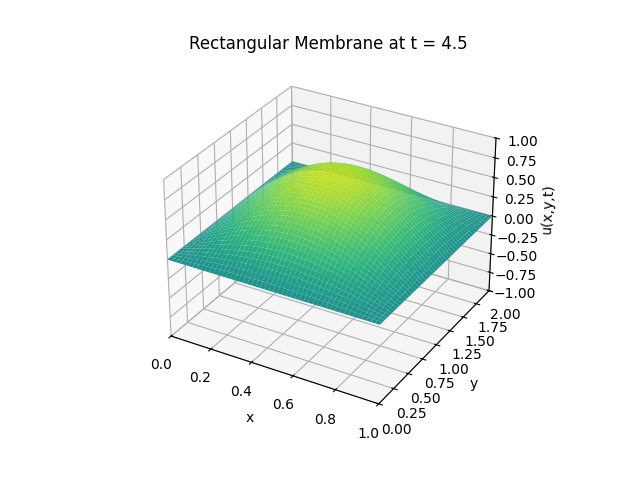
Visualising the solution for \(t \in [0, 6]\) with the partial sum
Animation:
Click to expand code
import matplotlib.pyplot as plt
import numpy as np
from matplotlib.animation import FuncAnimation


def rectangular_membrane_2(a: float = 1, b: float = 2, c: float = np.pi, tmax: int = 6):
    t = np.linspace(0, tmax, 100)  # Time points for animation
    x = np.linspace(0, a, 50)  # x grid
    y = np.linspace(0, b, 50)  # y grid
    X, Y = np.meshgrid(x, y)

    # Define the solution function
    def solution(x, y, t):
        z = 0
        for n in range(1, 31):
            for m in range(1, 31):
                lambda_nm = np.pi**2 * (n**2 / a**2 + m**2 / b**2)
                # Compute the coefficient Anm
                xx = np.linspace(0, a, 100)
                yy = np.linspace(0, b, 100)
                Anm = (
                    4
                    * np.trapezoid(
                        np.cos(np.pi / 2 + np.pi * xx / a) * np.sin(n * np.pi * xx / a),
                        xx,
                    )
                    * np.trapezoid(
                        np.cos(np.pi / 2 + np.pi * yy / b) * np.sin(m * np.pi * yy / b),
                        yy,
                    )
                    / (a * b)
                )
                z += (
                    Anm
                    * np.cos(c * np.sqrt(lambda_nm) * t)
                    * np.sin(n * np.pi * x / a)
                    * np.sin(m * np.pi * y / b)
                )
        return z

    # Set up the figure and axis for animation
    fig = plt.figure()
    ax = fig.add_subplot(111, projection="3d")
    ax.set_xlim(0, a)
    ax.set_ylim(0, b)
    ax.set_zlim(-1, 1)
    ax.set_xlabel("x")
    ax.set_ylabel("y")
    ax.set_zlabel("u(x,y,t)")
    ax.set_title("Rectangular Membrane")

    # Update function for FuncAnimation
    def update(frame):
        ax.clear()
        Z = solution(X, Y, frame)  # Compute the new Z values
        ax.plot_surface(X, Y, Z, cmap="viridis", vmin=-1, vmax=1)
        ax.set_xlim(0, a)
        ax.set_ylim(0, b)
        ax.set_zlim(-1, 1)
        ax.set_xlabel("x")
        ax.set_ylabel("y")
        ax.set_zlabel("u(x,y,t)")
        ax.set_title("Rectangular Membrane")

    # Create and save the animation
    anim = FuncAnimation(fig, update, frames=t, interval=50)
    anim.save("rectangular_membrane_2_animation.gif", writer="imagemagick", fps=20)

    plt.show()
Snapshots:

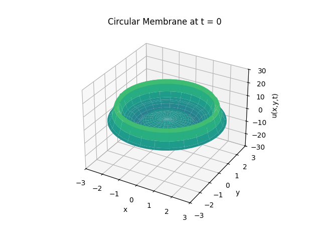
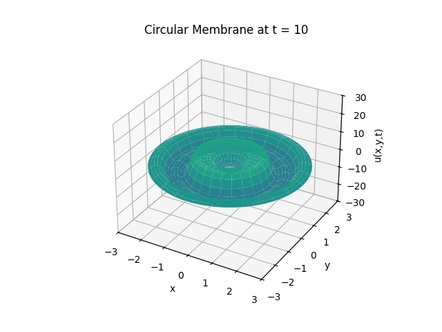
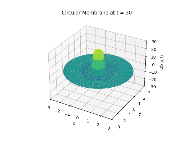
Circular Membrane
Pass
Fourier method: Change to polar coordinates
...
Then the function in the first initial condition \(u |_{t=0}\) becomes
which is radially symmetric and hence the solution will be also radially symmetric. It is given by
where
and \(\mu_m^{(0)}\) are the positive solutions to \(J_0(\mu) = 0\).
...

...
Animation:
Click to expand code
import matplotlib.pyplot as plt
import numpy as np
from matplotlib.animation import FuncAnimation
from scipy.optimize import root_scalar
from scipy.special import jv as besselj


def CircularMembrane(a=0.5, r=3, tmax=30, N=40):
    rho = np.linspace(0, r, 51)  # Radial grid points
    phi = np.linspace(0, 2 * np.pi, 51)  # Angular grid points
    t = np.linspace(0, tmax, 100)  # Time steps

    # Find the first 40 positive zeros of the Bessel function J0
    mju = []
    for n in range(1, N + 1):
        zero = root_scalar(
            lambda x: besselj(0, x), bracket=[(n - 1) * np.pi, n * np.pi]
        )
        mju.append(zero.root)
    mju = np.array(mju)

    # Define the initial position function
    def tau(rho):
        return rho**2 * np.sin(np.pi * rho) ** 3

    # Compute the solution for given R and t
    def solution(R, t):
        y = np.zeros_like(R)
        for m in range(N):
            s = tau(R[0, :]) * R[0, :] * besselj(0, mju[m] * R[0, :] / r)
            A0m = 4 * np.trapezoid(s, R[0, :]) / ((r**2) * (besselj(1, mju[m]) ** 2))
            y += A0m * np.cos(a * mju[m] * t / r) * besselj(0, mju[m] * R / r)
        return y

    # Create a grid of points
    R, p = np.meshgrid(rho, phi)
    X = R * np.cos(p)
    Y = R * np.sin(p)

    # Set up the figure and axis for animation
    fig = plt.figure()
    ax = fig.add_subplot(111, projection="3d")
    ax.set_xlim(-r, r)
    ax.set_ylim(-r, r)
    ax.set_zlim(-30, 30)
    ax.set_xlabel("x")
    ax.set_ylabel("y")
    ax.set_zlabel("u(x,y,t)")
    ax.set_title("Circular Membrane")

    # Update function for animation
    def update(frame):
        ax.clear()
        Z = solution(R, frame)
        ax.plot_surface(X, Y, Z, cmap="viridis", vmin=-30, vmax=30)
        ax.set_xlim(-r, r)
        ax.set_ylim(-r, r)
        ax.set_zlim(-30, 30)
        ax.set_title("Circular Membrane")
        ax.set_xlabel("x")
        ax.set_ylabel("y")
        ax.set_zlabel("u(x,y,t)")

    # Create and save the animation
    anim = FuncAnimation(fig, update, frames=t, interval=50)
    anim.save("circular_membrane_animation.gif", writer="imagemagick", fps=20)

    plt.show()
Snapshots: