In this post we are going to explore the Fourier method for solving the 1D and 2D wave equations. The method is more known under the name of the method of separation of variables. For the 1D wave equation we are going to show the application of the method to a fixed string, and for the 2D wave equation we are going to apply the method to a rectangular membrane and a circular membrane. We are also going to attempt to outline the physical interpretations of all scenarios.

1D Wave Equation

The 1D wave equation is of the form

$$ u_{tt} = a^2 u_{xx}. $$

Fixed String

First, let's take a look at the model of a string with length $l$ which is also fixed at both ends:

\begin{equation} \left\{\begin{aligned} u_{tt} = a^2 u_{xx}, \\ u(x, 0) = \varphi_1(x),\\ u_t(x, 0) = \varphi_2(x), \\ u(0, t) = u(l, t) = 0. \end{aligned}\right. \end{equation}

A visualisation of the string can be seen in the figure below.

We start solving the equation by taking into account only the boundary conditions $u(0, t) = u(l, t) = 0$. The idea is to find solution $u(x, t)$ of the form

$$ u(x, t) = X(x)T(t). $$

We substitute this form of the solution into the wave equation and get

$$ \frac{1}{a^2} T^{\prime\prime}(t)X(x) = T(t)X^{\prime\prime}(x), $$

further divding by $X(x)T(t)$ leads to

$$ \frac{1}{a^2} \frac{T^{\prime\prime}(t)}{T(t)} = \frac{X^{\prime\prime}(x)}{X(x)}. $$

We have two functions of independent variables which are equal. This is only possible if they are equal to the same constant. Therefore, let

$$ \frac{1}{a^2} \frac{T^{\prime\prime}(t)}{T(t)} = \frac{X^{\prime\prime}(x)}{X(x)} = -\lambda, $$

producing the following two equeations:

$$ T^{\prime\prime}(t) + a^2 \lambda T(t) = 0 $$

and

$$\label{eq:ref} X^{\prime\prime}(x) + \lambda X(x) = 0. \tag{*} $$

Let's begin with solving the second equation. The boundary conditions give

$$ X(0)T(t) = 0 \quad \text{and} \quad X(l)T(t) = 0. $$

Because we are interested only in non-trivial solutions and thus $T \neq 0$, we have

$$\label{eq:ref2} X(0) = 0 \quad \text{and} \quad X(l) = 0. \tag{**} $$

Now, we have to find the non-trivial solutions for $X(x)$ satisfying

$$ \left\{\begin{align*} X^{\prime\prime}(x) + \lambda X(x) = 0, \\ X(0) = 0, \quad X(l) = 0. \end{align*}\right. $$

The above problem is an example of the so called Sturm-Liouville problem. In order to find the general solution of the second order linear homogeneous differential equation with constant coefficients $\eqref{eq:ref}$ we should solve its characteristic equation

$$ r^2 + \lambda = 0. $$

If $\lambda < 0$, then $r_{1, 2} = \pm \sqrt{-\lambda}$, hence the general solution is
$$ X(x) = c_1 e^{\sqrt{-\lambda}x} + c_2 e^{-\sqrt{-\lambda}x} $$
for some constants $c_1$ and $c_2$. In order to determine the constants we substitute the above solution into the boundary conditions $\eqref{eq:ref2}$ and get the system
$$ \left\{\begin{align*} c_1 + c_2 = 0, \\ c_1 e^{\sqrt{-\lambda}l} + c_2 e^{-\sqrt{-\lambda}l} = 0. \end{align*}\right. $$
This results in $c_1 = c_2 = 0$, meaning our Sturm-Liouville problem doesn't have a non-zero solution for $\lambda < 0$.
If $\lambda = 0$, then $r_1 = r_2 = 0$ and the general solution is
$$ X(x) = c_1 + c_2 x. $$
Substituing it into the boundary conditions $\eqref{eq:ref2}$ again lead to $c_1 = c_2 = 0$, hence no non-zero solutions of our Sturm-Liouville problem for $\lambda \leq 0$.
If $\lambda > 0$, then $r_{1, 2} = \pm i \sqrt{\lambda}$, and the general solution becomes
$$ X(x) = c_1 \cos{\left( \sqrt{\lambda} x \right)} + c_2 \sin{\left(\sqrt{\lambda}x\right)}. $$
Substituting into the boundary conditions $\eqref{eq:ref2}$ results in
$$ \left\{\begin{align*} c_1 = 0, \\ c_2 \sin{\left(\sqrt{\lambda}l\right)} = 0 \end{align*}\right. $$
If $c_2 = 0$, then $X(x) \equiv 0$ which is a trivial solution. Therefore, we set $c_2 \neq 0$ and hence
$$ \sin{\left(\sqrt{\lambda}l\right)} = 0, $$
giving $\sqrt{\lambda}l = k \pi$, $k = \pm 1, \pm 2, ...$. Theerfore,
$$ \lambda = \lambda_k = \left(\frac{k \pi}{l}\right)^2, $$
meaning eigenvalues exist when $\lambda > 0$. The eigenfunctions corresponding to the above eigenvalues are
$$ X_k(x) = \sin{\left(\frac{k \pi x}{l}\right)}, \quad k > 0, k \in N. $$

Going back to $T^{\prime\prime}(t) + a^2 \lambda T(t) = 0$, solving in analogical way, when $\lambda = \lambda_k$ the solution becomes

$$ T_k(t) = A_k \cos{\left(\frac{ak\pi}{l}t\right)} + B_k \sin{\left(\frac{ak\pi}{l}t\right)} $$

for some constants $A_k$ and $B_k$. Hence,

$$ u_k(x,t) = X_k(x) T_k(t) = \left(A_k \cos{\left(\frac{ak\pi}{l}t\right)} + B_k \sin{\left(\frac{ak\pi}{l}t\right)}\right) \sin{\left(\frac{k \pi x}{l}\right)}, \quad k > 0, k \in N $$

are solutions to our wave equation, also satisfying the boundary conditions. Since our equation is linear, forming a linear system with its conditions, the principle of superposition is valid. In other words, if $u_1, u_2, ..., u_n$ are solutions of our system, then

$$ \alpha_1 u_1 + \alpha_2 u_2 + ... + \alpha_n u_n $$

for some constants $\alpha_1, \alpha_2, ..., \alpha_n$ is also a solution of the system. But in our case we have an infinite number of functions $u_1, u_2, ...$ which satisfy the linear system. Therefore, we need the generalised superposition principle stating that in such case

$$ u = \sum_n^{\infty} \alpha_n u_n $$

for some arbitrary constants $\alpha_n$ is a solution to the system if the series converges uniformly and is twice differentiable termwise. This generalisation is a Lemma and should be prooved. The proof can be found in ...

Assuming we have prooved the said Lemma, we can state that our system has a solution of the form

$$ u(x, t) = \sum_{k=1} ^{\infty} u_k(x, t) = \sum_{k=1}^{\infty} \left(A_k \cos{\left(\frac{ak\pi}{l}t\right)} + B_k \sin{\left(\frac{ak\pi}{l}t\right)}\right) \sin{\left(\frac{k \pi x}{l}\right)}. $$

The next task we have to tackle is to determine the coefficients $A_k$ and $B_k$. We can achieve this by using the initial conditions

$$ u(x, 0) = \varphi_1(x), \quad \text{and} \quad u_t(x, 0) = \varphi_2(x). $$

We get

$$ u(x, 0) = \sum_{k=1} ^{\infty} A_k \sin{\left(\frac{k \pi x}{l}\right)} = \varphi_1(x) $$

and

$$ u_t(x, 0) = \sum_{k=1}^{\infty} \frac{ak\pi}{l} B_k \sin{\left(\frac{k \pi x}{l}\right)} = \varphi_2(x). $$

Now, we have to expand both $\varphi_1(x)$ and $\varphi_2(x)$ into series in terms of sines only (why?). We have

$$ \varphi_1(x) = \sum_{k=1}^{\infty} \varphi_k^{(1)} \sin{\left(\frac{k \pi}{l}x\right)} $$

and

$$ \varphi_2(x) = \sum_{k=1}^{\infty} \varphi_k^{(2)} \sin{\left(\frac{k \pi}{l}x\right)}. $$

By the Fourier series theroem of uniqueness, we get

$$ A_k = \varphi_k^{(1)} \quad \text{and} \quad B_k = \frac{l}{ak\pi} \varphi_k^{(2)}, $$

or (why?)

$$ A_k = \frac{2}{l} \int_{0}^{l} \varphi_1(x) \sin{\left(\frac{k \pi}{l}x\right)} \mathrm{d}x $$

and

$$ B_k = \frac{2}{ak\pi} \int_{0}^{l} \varphi_2(x) \sin{\left(\frac{k \pi}{l}x\right)} \mathrm{d}x. $$

We are left with the task of the covergence of the infinite series. We have to explore the following series

$$ |u(x, t)| \leq \sum_{k=1}^{\infty}(|A_k| + |B_k|), $$

$$ |u_t(x, t)| \leq \sum_{k=1}^{\infty}\frac{ak\pi}{l}(|A_k| + |B_k|), $$

$$ |u_x(x, t)| \leq \sum_{k=1}^{\infty}\frac{k\pi}{l}(|A_k| + |B_k|), $$

$$ |u_{tt}(x, t)| \leq \sum_{k=1}^{\infty}\frac{a^2 k^2 \pi^2}{l^2}(|A_k| + |B_k|), $$

$$ |u_{xx}(x, t)| \leq \sum_{k=1}^{\infty}\frac{k^2 \pi^2}{l^2}(|A_k| + |B_k|). $$

If the series on the right side (majorizing series) converge then the series on the left would also converge and the needed differentiation would exist. It is enough (why?) for the following series to converge

$$ \sum_{k=1}^{\infty} k^j \left(|\varphi_k^{(1)}| + \frac{2}{ak\pi}|\varphi_k^{(2)}|\right), j = 0, 1, 2. $$

This is possible only if

$$ \left\{\begin{align*} \sum_{k=1}^{\infty} k^j |\varphi_k^{(1)}|, \\ \sum_{k=1}^{\infty} k^{j-1} |\varphi_k^{(2)}|, \end{align*}\right. \quad j = 0, 1, 2. $$

converge. From Calculus we know (theorem) that if $\varphi(x)$ is $m$-times differentiable then

$$ \sum_{k=1}^{\infty} k^{m-1} |\varphi_k| $$

convergres. Therefore, in order for all the majorzing series to converge it is enough $\varphi_1(x)$ to be $3$-times differentiable, and $\varphi_2(x)$ to be $2$-times differentiable.

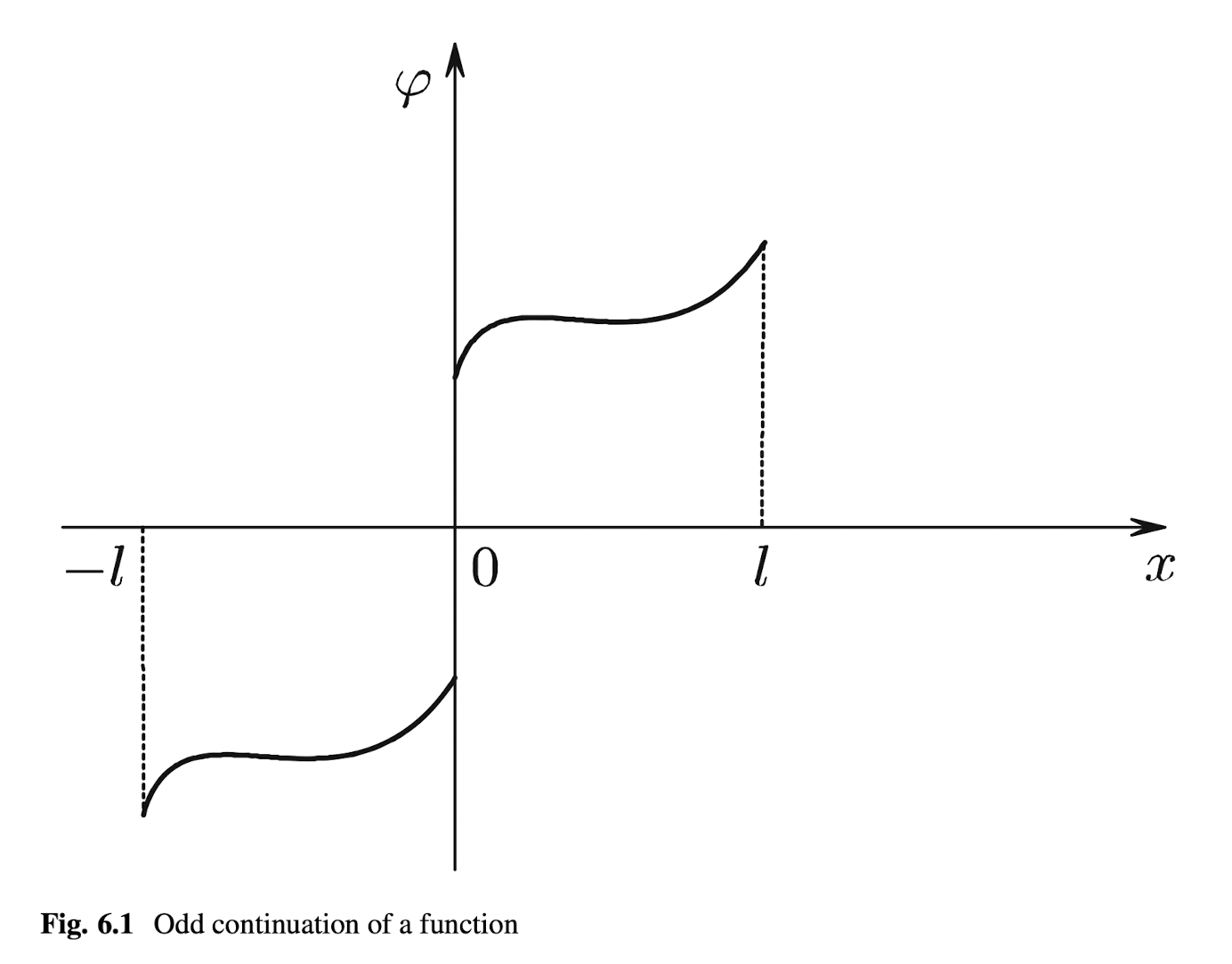
Finally, we should note a few things about the expansion of $\varphi_1(x)$ and $\varphi_2(x)$ into sine series. We have to note that in order to do that the function needs to be continued as an odd function which my lead to loss of the regularity of the lower derivatives. Let $\tilde{\varphi}_1(x)$ be the continuation of $\varphi_1(x)$ as an odd function (see the Figure below) defined as

$$ \tilde{\varphi}_1(x) = \left\{\begin{align*} \varphi_1(x), \quad 0 \leq x \leq l, \\ -\varphi_1(-x), \quad -l \leq x \leq 0. \end{align*}\right. $$

Hence, in order for it to be continous and continously differentibale we need to enforce the following condition

$$ \varphi_1(0) = \varphi_1(l) = 0. $$

To summarise, in order for $\sum_{k=1}^{\infty} \varphi_k^{(1)} \sin{\left( \frac{k\pi}{l}x\right)}$ to converge in $[0, l]$ it is necessary to enforce the above conditions to have zero values at both ends of the interval. As for the second derivative, if it exists it would be continuous as well. Similarly, for the third derivative to exist we enforce

$$ \varphi_1^{\prime\prime}(0) = \varphi_1^{\prime\prime}(l) = 0 $$

and obtain the corresponding necessary condition

$$ \varphi_2(0) = \varphi_2(l) = 0. $$

Finally, after these enforced conditions we can conclude that (tehorem)

$$ u(x, t) = \sum_{k=1}^{\infty} \left(A_k \cos{\left(\frac{ak\pi}{l}t\right)} + B_k \sin{\left(\frac{ak\pi}{l}t\right)}\right) \sin{\left(\frac{k \pi x}{l}\right)} $$

is a regular solution of the problem.

Physical interpretation:

If we go back to the eigenfunction

$$ u_k(x,t) = \left(A_k \cos{\left(\frac{ak\pi}{l}t\right)} + B_k \sin{\left(\frac{ak\pi}{l}t\right)}\right) \sin{\left(\frac{k \pi}{l}x\right)}, \quad k > 0, k \in N $$

we can rewrite it as

$$ u_k(x,t) = \sqrt{A_k^2 + B_k^2} \sin{\left(\frac{k \pi}{l}x\right)} \sin{\left(\frac{ak\pi}{l}t + \phi_k\right)}, \quad k \in N, $$

where

$$ \tan{(\phi_k)} = \frac{A_k}{B_k}. $$

We can translate this as the points of the string to oscillate at the frequency $\omega_k = \frac{ak\pi}{l}$ with phase $\phi_k$. The amplitude is dependant on $x$ and is given by

$$ F_k = \sqrt{A_k^2 + B_k^2} \sin{\left(\frac{k\pi}{l}x\right)}. $$

The $u_k(x, t)$ waves are called standing-waves. Depending on the values of $k$ we have the following scenarios:

When $k = 1$ there are $2$ motionless points which are the ends of the (fixed) string
When $k = 2$ a third moitonless point $x = \frac{l}{2}$ is added

These motionless points are called nodes of the standing wave. In general, $u_k(x, t)$ has $(k + 1)$ nodes located ate $0, \frac{1}{k}l, \frac{2}{k}l, ..., \frac{k-1}{k}l, l$. The maximum amplitude is achieved in the middle points between two nodes. These points are called crests. The fundamental tone, or the lowest tone, has frequency of $\omega_1 = \frac{a\pi}{l}$. The frequencies $\omega_k$ are called harmonics, while the higher tones corresponding to $\omega_k$, $k = 2, 3, ...$ are called overtones. It is quite natural to notice that the higher the value of $k$ the rapidly lower the amplitude of $u_k(x, t)$ becomes. Meaning, the effect from the higher harmonics all combined influences the quality of the sound. The below figure shows the harmonics for $k = 1, 2, 3$.

2D Wave Equation

The 2D wave equation is of the form

$$\label{eq:tdwave} \frac{\partial^2 u}{\partial t^2} = a^2 \Delta{u} = a^2\left(\frac{\partial^2 u}{\partial^2 x^2} + \frac{\partial^2 u}{\partial y^2}\right). \tag{1} $$

Rectangular Membrane

Let's assume we have a rectangular membrane with sides of length $l_1$ and $l_2$. Let's also assume it is fastened along the edges. A visaulisation can be seen below.

We can describe the problem via the model

$$ \left\{\begin{align*} \frac{\partial^2 u}{\partial t^2} = a^2 \Delta{u} = a^2\left(\frac{\partial^2 u}{\partial^2 x^2} + \frac{\partial^2 u}{\partial y^2}\right), \quad 0 < x < l_1, \quad 0 < y < l_2, \\ u|_{\Gamma} = 0, \\ u|_{t=0} = \varphi(x, y), u_t|_{t=0} = \psi(x, y), \end{align*}\right. $$

also with boundary conditions coming from the rectangular boundary $\Gamma$

$$ \left\{\begin{align*} u(0, y, t) = 0, \quad u(x, 0, t) = 0, \\ u(l_1, y, t) = 0, \quad u(x, l_2, t) = 0. \end{align*}\right. $$

A visualisation of the problem can be seen below.

As in the 1D wave equation, we are going to apply the Fourier method, meaning we are looking for a solution of the form

$$ U(x, y, t) = T(t)W(x, y). $$

Substituting into the 2D wave equation $\eqref{eq:tdwave}$ we get

$$ T^{\prime\prime}W = a^2 T \Delta{W}. $$

Then, we divide by $a^2TW$ and get

$$ \frac{T^{\prime\prime}}{a^2T} = \frac{\Delta{W}}{W} = - \lambda^2, $$

leading to the following equations

$$ T^{\prime\prime} + \lambda^2 a^2 T = 0 $$

and

$$ \Delta{W} + \lambda^2 W = 0. \quad \text{(Helmholtz equation)} $$

Now, we should do the same and apply the Fourier method to the Helmoltz equation. We are looking for a solution of the form

$$ W(x, y) = X(x) Y(y). $$

Substitution leads to

$$ X^{\prime\prime}Y + XY^{\prime\prime} + \lambda^2 XY = 0. $$

Further, dividing by $XY$ gives

$$ -\frac{X^{\prime\prime}}{X} = \frac{Y^{\prime\prime}}{Y} + \lambda^2 = \alpha^2. $$

Once again, we obtain the following to equations

$$ X^{\prime\prime} + \alpha^2 X = 0, $$

and

$$ Y^{\prime\prime} + \beta^2Y = 0, $$

where

$$ \lambda^2 = \alpha^2 + \beta^2. $$

Now, the boundary conditions take the forms

$$ X(0) Y(y) T(t) = 0, \quad \text{and} \quad X(l_1) Y(y) T(t) = 0, $$

and because we are looking for non-trivial solutions meaning $T(t) \neq 0$ and $Y(y) \neq 0$ identically, it follows

$$ X(0) = X(l_1) = 0. $$

Now, with the same logic first we have the boundary conditions

$$ X(x)Y(0)T(t) = 0, \quad \text{and} \quad X(x)Y(l_2)T(t) = 0, $$

then since $X(x) \neq 0$, and $T(t) \neq 0$ it follows

$$ Y(0) = Y(l_2) = 0. $$

We obtain the following Sturm-Liouville problms

$$ \left\{\begin{align*} X^{\prime\prime} + \alpha^2 X = 0, \\ X(0) = X(l_1) = 0, \end{align*}\right. $$

and

$$ \left\{\begin{align*} Y^{\prime\prime} + \beta^2Y = 0, \\ Y(0) = Y(l_2) = 0, \end{align*}\right. $$

with eigenvalues and corresponing eigenfunctions, respectively,

$$ \alpha_k = \frac{k\pi}{l_1}, k = 1,2,..., \quad X_k(x) = \sin{\left(\frac{k\pi}{l_1}x\right)} $$

and

$$ \beta_k = \frac{n\pi}{l_2}, n = 1,2,..., \quad Y_n(y) = \sin{\left(\frac{n\pi}{l_2}y\right)}. $$

As defined earlier, to every pair $\alpha_k$, $\beta_k$ there is a corresponding $\lambda_{kn}^2 = \alpha_k^2 + \beta_k^2$. This is a Dirichlet eigenvalue of the Laplacian in our rectangular membrane. For each $\lambda_{kn}$ we have

$$ \lambda_{kn} = \sqrt{\alpha_k^2 + \beta_k^2} = \pi \sqrt{\frac{k^2}{l_1^2} + \frac{n^2}{l_2^2}} $$

and hence the corresponding general solution of $T^{\prime\prime} + \lambda_{kn}^2 a^2 T = 0$ is

$$ T_{kn}(t) = A_{kn}\cos{(a\lambda_{kn}t)} + B_{kn}\sin{(a\lambda_{kn}t)}. $$

Again, by the superposition principle, the solution of our 2D wave equation on rectangular membrane is sought in the form

$$ u(x, y, t) = \sum_{k,n=1}^{\infty}\left(A_{kn}\cos{(a\lambda_{kn}t)} + B_{kn}\sin{(a\lambda_{kn}t)}\right)\sin{\left(\frac{k\pi}{l_1}x\right)}\sin{\left(\frac{n\pi}{l_2}y\right)}. $$

...

$$ u(x, y, 0) = \sum_{k,n=1}^{\infty}A_{kn}\sin{\left(\frac{k\pi}{l_1}x\right)}\sin{\left(\frac{n\pi}{l_2}y\right)} = \varphi(x, y), $$

and

$$ u_t(x, y, 0) = \sum_{k,n=1}^{\infty}B_{kn}a\lambda_{kn}\sin{\left(\frac{k\pi}{l_1}x\right)}\sin{\left(\frac{n\pi}{l_2}y\right)} = \psi(x, y). $$

...

$$ \omega_{kn}(x, y) := \sin{\left(\frac{k\pi}{l_1}x\right)}\sin{\left(\frac{n\pi}{l_2}y\right)} $$

...

$$ \int_0^{l_1} \int_0^{l_2} \omega_{kn}(x, y) \omega_{rs}(x, y) \mathrm{d}x \mathrm{d}y = \left\{\begin{align*} 0, \quad k \neq r \quad \text{or} \quad n \neq s, \\ \frac{l_1 l_2}{4}, \quad k = r \quad \text{and} \quad n = s. \end{align*}\right. $$

...

$$ A_{kn} = \frac{4}{l_1 l_2} \int_0^{l_1} \int_0^{l_2} \varphi(x, y) \sin{\left(\frac{k\pi}{l_1}x\right)} \sin{\left(\frac{n\pi}{l_2}y\right)} \mathrm{d}x \mathrm{d}y, $$

and

$$ B_{kn} = \frac{4}{l_1 l_2 a \lambda_{kn}} \int_0^{l_1} \int_0^{l_2} \psi(x, y) \sin{\left(\frac{k\pi}{l_1}x\right)} \sin{\left(\frac{n\pi}{l_2}y\right)} \mathrm{d}x \mathrm{d}y. $$

Circular Membrane

Let's assume we have a circular membrane with radius of length $\rho$. Let's also assume it is fastened along the edges. A visaulisation can be seen below.

... the polar change of coordinates

$$ \left\{\begin{align*} x = \rho \cos{(\varphi)}, \\ y = \rho \sin{(\varphi)}. \end{align*}\right. $$

A visualisation of the polar change can be seen below.

Now, let's ...

$$ \frac{\partial^2 u}{\partial t^2} = a^2 \Delta{u} = a^2\left(\frac{\partial^2 u}{\partial^2 x^2} + \frac{\partial^2 u}{\partial y^2}\right) $$

$$ x^2 + y^2 = \rho^2 (\cos^2{(\varphi)} + \sin^2{(\varphi)}) = \rho^2, \\ \rho = \sqrt{x^2 + y^2} $$

and

$$ \frac{y}{x} = \frac{\rho \sin{(\varphi)}}{\rho \cos{(\varphi)}} = \tan{(\varphi)}, \\ \varphi = \arctan{\left(\frac{y}{x}\right)} $$

$$ u = u(x, y, t) \quad \text{becomes} \quad u(\rho(x, y), \varphi(x, y), t) $$

First partial derivative, Chain rule

$$ \frac{\partial u}{\partial x} = \frac{\partial u}{\partial \rho} \frac{\partial \rho}{\partial x} + \frac{\partial u}{\partial \varphi} \frac{\partial \varphi}{\partial x}, $$

and

$$ \frac{\partial u}{\partial y} = \frac{\partial u}{\partial \rho} \frac{\partial \rho}{\partial y} + \frac{\partial u}{\partial \varphi} \frac{\partial \varphi}{\partial y}. $$

Now, for $\rho$

$$ \frac{\partial \rho}{\partial x} = \frac{1}{2} \frac{1}{\sqrt{(x^2 + y^2)}} (2x) = \frac{x}{\rho} = \cos{(\varphi)}, $$

$$ \frac{\partial \rho}{\partial y} = \frac{1}{2} \frac{1}{\sqrt{(x^2 + y^2)}} (2y) = \frac{y}{\rho} = \sin{(\varphi)}, $$

and for $\varphi$

$$ \frac{\partial \varphi}{\partial x} = \frac{1}{1 + \left(\frac{y}{x}\right)^2} y \left(-\frac{1}{x^2}\right) = -\frac{y}{x^2 + y^2} = - \frac{\rho \sin{(\varphi)}}{\rho^2} = - \frac{\sin{(\varphi)}}{\rho}, $$

$$ \frac{\partial \varphi}{\partial y} = \frac{1}{1 + \left(\frac{y}{x}\right)^2} \left(\frac{1}{x}\right) = \frac{x}{x^2 + y^2} = \frac{\rho \cos{(\varphi)}}{\rho^2} = \frac{\cos{(\varphi)}}{\rho}. $$

Therefore,

$$ \frac{\partial u}{\partial x} = \cos{(\varphi)} \frac{\partial u}{\partial \rho} - \frac{\sin{(\varphi)}}{\rho} \frac{\partial u}{\partial \varphi}, $$

$$ \frac{\partial u}{\partial y} = \sin{(\varphi)} \frac{\partial u}{\partial \rho} + \frac{\cos{(\varphi)}}{\rho} \frac{\partial u}{\partial \varphi}. $$

Second order derivatives

$$ \frac{\partial^2 u}{\partial x^2} = ... $$

...

A visualisation of the problem can be seen below.

...

JoJo's Blog

Fourier Method for the Wave Equation

1D Wave Equation

Fixed String

2D Wave Equation

Rectangular Membrane

Circular Membrane

1D Wave Equation

Fixed String

2D Wave Equation

Rectangular Membrane

Circular Membrane

links

social