In this post, we are going to explore Google’s PaliGemma 2 mix vision-language model (VLM), and its capabilities to perform image segmentation. What’s interesting is that we are going to perform this task by only using Apple’s MLX framework, and MLX-VLM. This would eliminate the dependency of using JAX/Flax as in the original Google’s segmentation script, and would allow us to fully and seamlessly utilise Apple’s unified memory.

Introduction

PaliGemma 2

In December 2024 Google introduced the PaliGemma 2 vision-language models (VLMs). These are pre-trained (pt) models coming in three different sizes: 3B, 10B, and 28B, as well as three different input resolutions for images: 224x224, 448x448, and 896x896 pixels. These models represent the latest evolution of vision-language models developed by Google, building upon the foundation laid by its predecessor, PaliGemma. Below, we can see the architecture of the PaliGemma 2 model.

PaliGemma 2 architecture

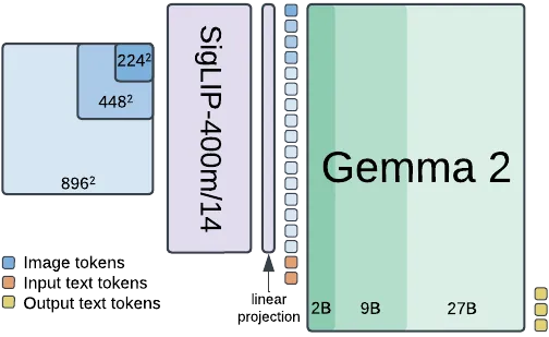
Figure 1 | PaliGemma 2 architecture; source: https://arxiv.org/pdf/2412.03555

PaliGemma 2 processes images at resolutions of 224×224, 448×448, or 896×896 pixels using a SigLIP-400m vision encoder with a patch size of 14×14 pixels. This design yields 256, 1024, or 4096 tokens, respectively. After a linear projection, the resulting image tokens are concatenated with the input text tokens, and Gemma 2 is used as a text decoder to autoregressively complete the combined prefix to generate an answer.

PaliGemma 2 Mix

As already mentioned, PaliGemma 2 models are pre-trained models, but they are also designed to be easy to fine-tune and adapt to various specific vision-language tasks and domains. Google wanted to demonstrate the performance of a fine-tuned version of the pt PaliGemma 2 models on downstream tasks, and thus a few months later, in February 2025, they introduced PaliGemma 2 mix. These models are fine-tuned to a mixture of vision language tasks that can be used out-of-the-box for common use cases. They are available in three sizes: 3B, 10B, and 28B, and support resolutions of 224×224 and 448×448 pixels.

Tasks

PaliGemma 2 mix can perform the following types of tasks:

Short and long captioning
Optical character recognition (OCR)
Image question answering
(Multiple) object detection
(Multiple) image segmentation

Prompting

In general, the PaliGemma models are very sensitive to the prompt’s syntax and patterns. But based on the following Hugging Face article when using PaliGemma 2 mix models, open-ended prompts yield better performance than the previously required task-prefixed prompts. Earlier, task-specific prefixes were essential, like

“caption {lang}\n”: Short captions
“describe {lang}\n”: More descriptive captions
“ocr”: Optical character recognition
“answer {lang} {question}\n”: Question answering about the image contents
“question {lang} {answer}\n”: Question generation for a given answer

However, two specific tasks — object detection and image segmentation — still exclusively require task prefixes:

"detect {object description} ; {object description} ; ...\n": Locate multiple objects in an image and return the bounding boxes for those objects
"segment {object description} ; {object description} ; ...\n": Locate the area occupied by multiple objects in an image to create an image segmentation for that object

Image Segmentation

What is Image Segmentation?

Image segmentation is a key computer vision technique that divides an image into pixel groups, or segments, enabling tasks like object detection, scene understanding, and advanced image processing. Traditional methods use pixel features such as color, brightness, contrast, and intensity to separate objects from the background, often relying on simple heuristics or basic machine learning. Recently, deep learning models with complex neural networks have dramatically improved segmentation accuracy.

Unlike image classification, which labels an entire image, or object detection, which locates objects with bounding boxes, image segmentation provides detailed pixel-level annotations. This approach assigns every pixel to a specific category, with variants including semantic segmentation (classifying pixels), instance segmentation (distinguishing between instances of the same object), and panoptic segmentation (combining both methods).

Image Segmentation with VLMs

VLMs enhance traditional image segmentation by enabling open-vocabulary segmentation through textual instructions, moving away from closed-set methods that rely on predefined categories. By merging text and image data into a common feature space, these models reduce adaptation costs and excel at tasks like referring expression segmentation. For example, a user might prompt the model to “segment the cat sitting on the chair”, and the VLM would identify and segment the pixels corresponding to that specific cat.

To achieve this, VLMs harness visual features from encoders like CNNs or Vision Transformers, using cross-attention to focus on image regions relevant to the text. Some models are fine-tuned to produce bounding boxes or segmentation masks directly, and careful prompting guides them to accurately segment based on the integrated understanding of visual content and language.

Image Segmentation the PaliGemma 2 Way

Earlier, in Figure 1 we saw that PaliGemma 2’s architecture combines a Transformer decoder based on the Gemma 2 language model with a Vision Transformer image encoder initialised from SigLIP-So400m/14. The SigLIP encoder divides input images into 14x14 pixel patches to generate “soft tokens” that capture spatial relationships. Then, a linear projection layer is used to map the visual tokens into the same dimensional space as the input embeddings of the Gemma 2 language model. This projection ensures that the visual information can be seamlessly combined with textual information for processing by the language model.

The Gemma 2 language model functions as the decoder, processing concatenated image tokens and text tokens to produce autoregressive text output, predicting one token at a time based on the preceding context. To enhance its capabilities for vision-language tasks, PaliGemma extends the vocabulary of the standard Gemma tokenizer (having 256,000 tokens) with additional special tokens. These include 1024 tokens representing coordinates in a normalised image space, denoted as through , and another 128 tokens, through , which are codewords used for a lightweight referring-expression segmentation vector-quantized approach.

Segmentation Output

When processing a segmentation prompt, PaliGemma 2 mix produces a sequence that begins with four location tokens defining the bounding box for the segmented object. These four tokens specify the bounding box coordinates in the normalized image space. This is followed by 16 segmentation tokens, which can be decoded via a learned codebook into a binary segmentation mask confined within the identified region. Below is an example output:

<loc0336><loc0049><loc0791><loc0941><seg106><seg074><seg114><seg081><seg082><seg028><seg018><seg037><seg120><seg073><seg061><seg125><seg045><seg059><seg052><seg084>

Segmentation Mask

If we want to further process the 16 segmentation tokens to generate a binary segmentation mask within the identified bounding box, we have to decode the segmentation tokens by using the Decoder from Google’s big vision repository related to the PaliGemma models. It is available in the following script. As we can see, the script uses JAX and Flax, and it is known that the Metal plug-in for JAX is still not fully supported as stated in the Accelerated JAX on Mac article. In the next part of this post, we are going to show not only how to reconstruct the binary mask with the help of the above script, but we are also going to show how to translate JAX/Flax to mlx so that we can fully utilise the unified memory in Apple’s chips.

Tutorial

In this section, we are going to generate a segmentation mask with the PaliGemma 2 mix model, specifically mlx-community/paligemma2–10b-mix-448–8bit, by using only the packages mlx-vlm and mlx. We are also going to overlay the mask on top of the image we are segmenting.

Overview of the Process

Let’s first begin by outlining the steps of the process for generating a segmentation mask. An illustrative diagram can be seen in Figure 2.

We start with passing a prompt to the model of the form “segment cat\n”, and the image we want to segment. This is our original image with dimensions x_orig by y_orig.
Then, the model’s image processor (SiglipImageProcessor) yields to an input image with dimensions x_input by y_input. In the PaliGemma 2 mix case this would be either 224x224 or 448x448, depending on the model we have chosen to use. In our case, it would be 448x448.
The model generates an output with 4 location coordinates and 16 segmentation tokens. The sequence corresponds to the y_min, x_min, y_max, x_max coordinates defining the bounding box. These coordinates should be normalised to an image size of 1024x1024 to obtain the bounding box coordinates of the object we want to segment with respect to the input image dimensions.

Figure 2 | Model input and bounding box coordinates

Now that we’ve defined the bounding box by its coordinates, let’s zoom in on its details as shown in Figure 3, and dicuss how we would overlay the segmentation mask on top of the image we are segmenting.

The model has returned the 16 segmentation tokens of the form . After decoding them via the codebook we end up reconstructing the segmentation mask. This mask has a size of 64x64 pixels.
Next, we need to map the segmentation mask onto the bounding box that was previously defined. This is accomplished using classical interpolation techniques to scale the mask to the bounding box’s dimensions.

Figure 3 | Mapping the 64x64 mask to the bounding box Once resized, the mask is aligned to fit within the bounding box. To overlay this mask on the original image, we create an empty array matching the dimensions of the input image and then replace the array values corresponding to the bounding box coordinates with those from the interpolated segmentation mask.

MLX

Finally, it’s time to dive into the coding section of this blog and focus specifically on the mlx components. The code can be found in GitHub. We begin by importing the necessary libraries and modules,

import argparse
import functools
import logging
import re
from typing import Callable, List, Tuple

import cv2
import matplotlib.pyplot as plt
import mlx.core as mx
import mlx.nn as nn
import numpy as np
from mlx_vlm import apply_chat_template, generate, load
from mlx_vlm.utils import load_image
from tensorflow.io import gfile

then, we establish the paths for the models and image resources. The MODEL_PATH points to the specific PaliGemma model that we are going to use for segmentation tasks. The IMAGE_PATH is the location of the image that we will process, and the _KNOWN_MODELS dictionary provides a reference to the VAE checkpoint needed for mask reconstruction.

MODEL_PATH = "mlx-community/paligemma2-10b-mix-448-8bit"
IMAGE_PATH = "https://huggingface.co/datasets/huggingface/documentation-images/resolve/main/transformers/tasks/car.jpg"
_KNOWN_MODELS = {"oi": "gs://big_vision/paligemma/vae-oid.npz"}

Before diving into the core functionality, we set up logging to keep track of the execution flow and for debugging purposes. The following snippet initializes Python’s built-in logging system:

logging.basicConfig()
log = logging.getLogger(__name__)
log.setLevel(logging.INFO)

The ResBlock class implements a basic residual block typical for convolutional architectures. It comprises three convolution layers:

Two 3x3 convolutions with ReLU activations, which process the input.
One 1x1 convolution to adjust dimensions if needed.

The output of the block is computed by summing the result of the convolutions with the original input. This residual connection helps maintain gradient flow during training and preserves information across layers.

class ResBlock(nn.Module):
    def __init__(self, features: int):
        super().__init__()
        self.conv1 = nn.Conv2d(
            in_channels=features, out_channels=features, kernel_size=3, padding=1
        )
        self.conv2 = nn.Conv2d(
            in_channels=features, out_channels=features, kernel_size=3, padding=1
        )
        self.conv3 = nn.Conv2d(
            in_channels=features, out_channels=features, kernel_size=1, padding=0
        )

    def __call__(self, x: mx.array) -> mx.array:
        original_x = x
        x = nn.relu(self.conv1(x))
        x = nn.relu(self.conv2(x))
        x = self.conv3(x)
        return x + original_x

The Decoder class takes quantized vectors (obtained from segmentation tokens) and upscales them to produce a mask:

An initial convolution reduces the channel dimension.
A series of configurable residual blocks further process the features. Multiple transpose convolution layers (upsample layers) scale the feature maps until the desired resolution is reached.
A final convolution produces the output mask.

class Decoder(nn.Module):
    """Decoder that upscales quantized vectors to produce a mask.
    The architecture is parameterized to avoid hardcoded layer definitions.
    Takes channels-last input data (B, H, W, C).
    """

    def __init__(
        self,
        in_channels: int = 512,
        res_channels: int = 128,
        out_channels: int = 1,
        num_res_blocks: int = 2,
        upsample_channels: Tuple[int, ...] = (128, 64, 32, 16),
    ):
        super().__init__()
        self.conv_in = nn.Conv2d(
            in_channels=in_channels, out_channels=res_channels, kernel_size=1, padding=0
        )
        self.res_blocks = [
            ResBlock(features=res_channels) for _ in range(num_res_blocks)
        ]
        self.upsample_layers = []
        out_up_ch = res_channels
        for ch in upsample_channels:
            self.upsample_layers.append(
                nn.ConvTranspose2d(
                    in_channels=out_up_ch,
                    out_channels=ch,
                    kernel_size=4,
                    stride=2,
                    padding=1,
                )
            )
            out_up_ch = ch
        self.conv_out = nn.Conv2d(
            in_channels=upsample_channels[-1],
            out_channels=out_channels,
            kernel_size=1,
            padding=0,
        )

    def __call__(self, x: mx.array) -> mx.array:
        x = nn.relu(self.conv_in(x))
        for block in self.res_blocks:
            x = block(x)
        for layer in self.upsample_layers:
            x = nn.relu(layer(x))

        return self.conv_out(x)

The helper function _get_params is designed to convert a PyTorch checkpoint into a format that MLX can work with. It does so by Transposing kernel weights to match the expected output format: from PyTorch’s format to MLX’s (Out, H, W, In) format. Organizing the parameters into a structured dictionary that reflects the architecture of the decoder, including the convolutional layers, residual blocks, and upsample layers. This organized set of parameters is then used to initialize the decoder network.

def _get_params(checkpoint: dict) -> dict:
    """Converts PyTorch checkpoint to MLX params (nested dict).
    Uses transpositions yielding (Out, H, W, In) format weights."""

    def transp(kernel: np.ndarray) -> mx.array:
        return mx.transpose(mx.array(kernel), (0, 2, 3, 1))

    def transp_transpose(kernel: np.ndarray) -> mx.array:
        intermediate = mx.transpose(mx.array(kernel), (1, 0, 2, 3))

        return mx.transpose(intermediate, (0, 2, 3, 1))

    def conv(name: str) -> dict:
        return {
            "bias": mx.array(checkpoint[f"{name}.bias"]),
            "weight": transp(checkpoint[f"{name}.weight"]),
        }

    def conv_transpose(name: str) -> dict:
        return {
            "bias": mx.array(checkpoint[f"{name}.bias"]),
            "weight": transp_transpose(checkpoint[f"{name}.weight"]),
        }

    def resblock(name: str) -> dict:
        return {
            "conv1": conv(f"{name}.0"),
            "conv2": conv(f"{name}.2"),
            "conv3": conv(f"{name}.4"),
        }

    params = {
        "_embeddings": mx.array(checkpoint["_vq_vae._embedding"]),
        "conv_in": conv("decoder.0"),
        "res_blocks": [
            resblock("decoder.2.net"),
            resblock("decoder.3.net"),
        ],
        "upsample_layers": [
            conv_transpose("decoder.4"),
            conv_transpose("decoder.6"),
            conv_transpose("decoder.8"),
            conv_transpose("decoder.10"),
        ],
        "conv_out": conv("decoder.12"),
    }

    return params

The function _quantized_values_from_codebook_indices takes the segmentation tokens (represented as codebook indices) and uses the embeddings from the codebook to retrieve the corresponding encoded representations. These values are reshaped to fit the expected dimensions (batch, height, width, channels) so that they are ready for processing by the decoder.

def _quantized_values_from_codebook_indices(
    codebook_indices: mx.array, embeddings: mx.array
) -> mx.array:
    batch_size, num_tokens = codebook_indices.shape
    expected_tokens = 16
    if num_tokens != expected_tokens:
        log.error(f"Expected {expected_tokens} tokens, got {codebook_indices.shape}")

    encodings = mx.take(embeddings, codebook_indices.reshape((-1,)), axis=0)

    return encodings.reshape((batch_size, 4, 4, embeddings.shape[1]))

The get_reconstruct_masks function loads the VAE checkpoint and initializes the decoder with the appropriate parameters. By extracting and setting up the necessary embeddings and decoder weights, this function returns another function (reconstruct_masks) that, when given segmentation tokens, decodes them into a binary segmentation mask.

@functools.cache
def get_reconstruct_masks(model: str) -> Callable[[mx.array], mx.array]:
    """Loads the checkpoint and returns a function that reconstructs masks
    from codebook indices using a preloaded MLX decoder.
    """
    checkpoint_path = _KNOWN_MODELS.get(model, model)
    with gfile.GFile(checkpoint_path, "rb") as f:
        checkpoint_data = dict(np.load(f))

    params = _get_params(checkpoint_data)
    embeddings = params.pop("_embeddings")
    log.info(f"VAE embedding dimension: {embeddings.shape[1]}")

    decoder = Decoder()
    decoder.update(params)

    def reconstruct_masks(codebook_indices: mx.array) -> mx.array:
        quantized = _quantized_values_from_codebook_indices(
            codebook_indices, embeddings
        )
        return decoder(quantized)

    return reconstruct_masks

The function extract_and_create_arrays parses a given string pattern for segmentation tokens. It extracts these token numbers, converts them into integers, and then wraps them in MLX arrays for further mask reconstruction processing.

def extract_and_create_arrays(pattern: str) -> List[mx.array]:
    """Extracts segmentation tokens from each object in the pattern and returns a list of MLX arrays."""
    object_strings = [obj.strip() for obj in pattern.split(";") if obj.strip()]

    seg_tokens_arrays = []
    for obj in object_strings:
        seg_tokens = re.findall(r"<seg(\d{3})>", obj)
        if seg_tokens:
            seg_numbers = [int(token) for token in seg_tokens]
            seg_tokens_arrays.append(mx.array(seg_numbers))

    return seg_tokens_arrays

The parse_bbox function interprets the model's output string to extract bounding box coordinates. Each detected object's location is denoted by a string format (<loc1234>). This function finds four numbers per object, corresponding to the box boundaries, and aggregates them into a list of bounding boxes.

def parse_bbox(model_output: str):
    entries = model_output.split(";")

    results = []
    for entry in entries:
        entry = entry.strip()
        numbers = re.findall(r"<loc(\d+)>", entry)
        if len(numbers) == 4:
            bbox = [int(num) for num in numbers]
            results.append(bbox)

    return results

The gather_masks function combines the reconstruction and bounding box parsing steps. For each object:

It reconstructs the mask from its codebook indices.
It obtains the corresponding bounding box coordinates.
It normalizes these coordinates relative to a target image resolution (448×448 in this example).
Each mask is then paired with its coordinates and stored in a list, making it straightforward to later overlay these onto the original image.

def gather_masks(output, codes_list, reconstruct_fn):
    masks_list = []

    target_width, target_height = 448, 448
    for i, codes in enumerate(codes_list):
        codes_batch = codes[None, :]
        masks = reconstruct_fn(codes_batch)
        mask_np = np.array(masks[0, :, :, 0], copy=False)

        y_min, x_min, y_max, x_max = parse_bbox(output)[i]
        x_min_norm = int(x_min / 1024 * target_width)
        y_min_norm = int(y_min / 1024 * target_height)
        x_max_norm = int(x_max / 1024 * target_width)
        y_max_norm = int(y_max / 1024 * target_height)

        masks_list.append(
            {
                "mask": mask_np,
                "coordinates": (x_min_norm, y_min_norm, x_max_norm, y_max_norm),
            }
        )

    return masks_list

The function plot_masks handles the visualization of the segmentation outcomes. It loads the original image and processes it for display. Two types of visualizations are provided:

Composite Overlay: All masks are combined and overlaid on the original image.
Reconstructed Mask: Each reconstructed mask is plotted next to the composite overlay.

Using OpenCV for mask resizing and Matplotlib for plotting, the function creates a series of subplots to clearly display both composite and individual mask overlays.

def plot_masks(args, processor, masks_list):

    image = load_image(args.image_path)
    img_array = processor.image_processor(image)["pixel_values"][0].transpose(1, 2, 0)
    img_array = (img_array * 0.5 + 0.5).clip(0, 1)

    full = np.ones((448, 448, 1)) * (-1)
    for mask_info in masks_list:
        mask_np = mask_info["mask"]
        x_min_norm, y_min_norm, x_max_norm, y_max_norm = mask_info["coordinates"]

        width = x_max_norm - x_min_norm
        height = y_max_norm - y_min_norm

        resized_mask = cv2.resize(
            mask_np, (width, height), interpolation=cv2.INTER_NEAREST
        )
        resized_mask = resized_mask.reshape((height, width, 1))

        full[y_min_norm:y_max_norm, x_min_norm:x_max_norm] = resized_mask

    n_masks = len(masks_list)
    _, axs = plt.subplots(1, n_masks + 1, figsize=(5 * (n_masks + 1), 6))

    axs[0].imshow(img_array)
    axs[0].imshow(full, alpha=0.5)
    axs[0].set_title("Mask Overlay")
    axs[0].axis("on")

    for i, mask_info in enumerate(masks_list, start=1):
        mask_np = mask_info["mask"]
        axs[i].imshow(mask_np)
        axs[i].set_title(f"Reconstructed Mask {i}")
        axs[i].axis("on")

    plt.tight_layout()
    plt.show()

The main function ties all the pieces together. It performs the following steps:

Loading: Reads the specified PaliGemma model and image.
Setup: Initializes the VAE checkpoint and extracts the reconstruction function.
Prompting: Formats the prompt using the processor and generates a segmentation output via the model.
Processing: Extracts segmentation tokens, reconstructs masks, and parses bounding box coordinates.
Visualization: Finally, it calls the plotting function to display the results.

This function serves as the central point where data processing, model inference, mask reconstruction, and visualization are integrated into one complete pipeline.

def main(args) -> None:
    log.info(f"Loading PaliGemma model: {args.model_path}")
    model, processor = load(args.model_path)
    config = model.config

    image = load_image(args.image_path)
    log.info(f"Image size: {image.size}")

    vae_path = _KNOWN_MODELS.get(args.vae_checkpoint_path, args.vae_checkpoint_path)
    reconstruct_fn = get_reconstruct_masks(vae_path)

    prompt = args.prompt.strip() + "\n"
    log.info(f"Using prompt: '{prompt.strip()}'")
    formatted_prompt = apply_chat_template(processor, config, prompt, num_images=1)

    log.info("Generating segmentation output...")
    output = generate(model, processor, formatted_prompt, image, verbose=False)
    log.info(f"Model output: {output}")

    codes_list = extract_and_create_arrays(output)
    log.info(f"Extracted codes: {codes_list}")

    log.info("Reconstructing mask from codes...")
    masks_list = gather_masks(output, codes_list, reconstruct_fn)

    log.info("Plotting masks...")
    plot_masks(processor, masks_list)

Finally, the script includes an entry point that parses command-line arguments. Users can specify the image path, the prompt for the segmentation task, the model path, and the VAE checkpoint path. Once these are provided via argparse, the main function is invoked to start the processing pipeline.

if __name__ == "__main__":
    parser = argparse.ArgumentParser(description="Vision tasks using PaliGemma 2 mix.")
    parser.add_argument(
        "--image_path", type=str, default=IMAGE_PATH, help="Path to the input image."
    )
    parser.add_argument(
        "--prompt", type=str, required=True, help="Prompt for the model."
    )
    parser.add_argument(
        "--model_path", type=str, default=MODEL_PATH, help="Path to the mlx model."
    )
    parser.add_argument(
        "--vae_checkpoint_path", type=str, default="oi", help="Path to the .npz file."
    )

    cli_args = parser.parse_args()
    main(cli_args)

Results

Let’s take a look at some examples and the segmentations we obtained from the model.

Single Object Segmentation

In this section, we are going to show to examples of single object segmentation.

Prompt:

“segment cow”

Image:

Original image of size 400x400

Model output:

<loc0410><loc0528><loc0884><loc1023><seg072><seg055><seg062><seg079><seg104><seg009><seg104><seg096><seg068><seg041><seg103><seg019><seg100><seg004><seg091><seg067>

Mask overlay and reconstructed mask:

Left: mask overlay onto the input image of size 448x448 | Right: reconstructed mask of size 64x64

Observation:

Based on the overlay image, the model manages to detect the precise location of the cow but struggles a bit with the detailed outlines of the cow. Looking only at the reconstructed mask would not persuade me that this is a cow.

Prompt:

“segment cat”

Image:

Original image of size 400x400

Model output:

<loc0060><loc0000><loc0920><loc0879><seg039><seg107><seg018><seg006><seg056><seg120><seg058><seg042><seg079><seg094><seg009><seg099><seg074><seg010><seg078><seg012>

Mask overlay and reconstructed mask:

Left: mask overlay onto the input image of size 448x448 | Right: reconstructed mask of size 64x64

Observation:

Based on the overlay image, the model manages to detect the precise location of the cat, and is generally doing a good job with the cat’s outlines.

Multiple Object Segmentation

It was tricky to find a working example for segmenting multiple objects, so there is only one example in this section. My observation is that the PaliGemma models are indeed very sensitive to the prompt formatting, and the 448–10B-8bit model might just not be powerful enough for the task of segmenting multiple objects.

Prompt:

“segment left wheel ; right wheel”

Image:

Original image of size 640x480

Model output:

<loc0591><loc0157><loc0794><loc0311> <seg092><seg004><seg044><seg092><seg120><seg061><seg029><seg120><seg090><seg023><seg021><seg090><seg015><seg041><seg044><seg073> right wheel ; <loc0586><loc0728><loc0794><loc0882> <seg092><seg004><seg089><seg092><seg120><seg048><seg054><seg038><seg119><seg029><seg021><seg090><seg095><seg041><seg044><seg073> right wheel

Mask overlay and reconstructed mask:

Left: masks overlay onto the input image of size 448x448 | Right: reconstructed masks of size 64x64

Observation:

Looking at the model output we can see that both segmentations are labeled as right wheel. Despite this, based on the overlay image, the model manages to detect the precise location of the wheels, and their outlines.

Conclusion

In summary, we implemented a unified segmentation pipeline by combining Google’s PaliGemma 2 Mix model with Apple’s MLX framework. Our workflow involved formatting segmentation prompts, preprocessing images, extracting segmentation tokens and bounding box coordinates, decoding these tokens into segmentation masks, and finally overlaying the masks on the original images.

For single object segmentation, the model generally performed well: it accurately localised the object areas, as evidenced by both the “cat” and the “cow” examples. However, the segmentation for the “cow” revealed some challenges with capturing fine details, indicating areas for potential refinement.

The multiple object segmentation proved challenging, as we struggled to find more than one working example that produced multiple segmentations. In our single example, the model demonstrated the ability to detect the general locations of objects — successfully identifying both wheels — but it also suffered from issues such as prompt sensitivity and duplicate labelling. This difficulty may be attributed to the inherent prompt sensitivity of the model or potential limitations of the specific model variant, particularly the 448–10B-8bit configuration. These observations suggest that either refining prompt structures or exploring more powerful models may be essential for reliably handling segmentation tasks involving multiple objects.

References

Introducing PaliGemma 2 mix: A vision-language model for multiple tasks
PaliGemma prompt and system instructions
PaliGemma 2 Mix — New Instruction Vision Language Models by Google
Welcome PaliGemma 2 — New vision language models by Google
Introducing PaliGemma 2: Powerful Vision-Language Models, Simple Fine-Tuning
PaliGemma 2: A Family of Versatile VLMs for Transfer

JoJo's Blog

Image Segmentation with PaliGemma 2 Mix and MLX

Introduction

PaliGemma 2

PaliGemma 2 Mix

Tasks

Prompting

Image Segmentation

What is Image Segmentation?

Image Segmentation with VLMs

Image Segmentation the PaliGemma 2 Way

Segmentation Output

Segmentation Mask

Tutorial

Overview of the Process

MLX

Results

Single Object Segmentation

Multiple Object Segmentation

Conclusion

References

Introduction

PaliGemma 2

PaliGemma 2 Mix

Tasks

Prompting

Image Segmentation

What is Image Segmentation?

Image Segmentation with VLMs

Image Segmentation the PaliGemma 2 Way

Segmentation Output

Segmentation Mask

Tutorial

Overview of the Process

MLX

Results

Single Object Segmentation

Multiple Object Segmentation

Conclusion

References

links

social