An implicit surface is easy to describe with an equation. A sphere, for example, is the set of points where \(x^2+y^2+z^2-r^2=0\). Turning that equation into vertices and faces is a different problem. We have to decide both where the vertices should go and which ones should be connected. Dual Contouring approaches these decisions separately: it fits a vertex to local tangent planes, then uses the grid's sign changes to construct the mesh.
The method was introduced by Tao Ju, Frank Losasso, Scott Schaefer, and Joe Warren in Dual Contouring of Hermite Data, presented at SIGGRAPH 2002. Its input includes surface intersection positions and normals, which together are called Hermite data. The normals are what let the method locate an edge or corner that lies between grid samples.
Let's develop the construction in two dimensions first, work through its least-squares problem, and then build an actual three-dimensional mesh.
Why Place a Vertex Inside a Cell?
Suppose a curve crosses two edges of a square cell. Marching Squares, the two-dimensional analogue of Marching Cubes, connects the crossing points with a segment in this simple configuration. If the curve bends sharply inside the cell, that segment cuts across the corner.
Now suppose we also know the normal at each crossing. Each normal determines a tangent line. Intersecting those lines gives us a candidate corner, even though the corner itself does not lie on a grid edge.
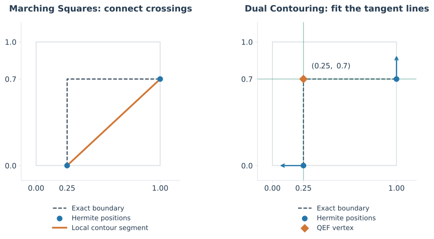
The same idea works in three dimensions, where tangent lines become tangent planes. Two independent planes locate a line; a third can locate a corner on that line.
The word dual refers to the exchange of roles between cells and mesh elements:
| Construction | In 2D | In 3D |
|---|---|---|
| Active grid cell | Supplies one contour vertex | Supplies one mesh vertex |
| Sign-changing interior grid edge | Supplies a segment joining two cell vertices | Supplies a quad joining four cell vertices |
These are the uniform-grid rules for the basic, one-vertex-per-cell version of Dual Contouring. Vertex positions and connectivity come from different information: tangent constraints determine the first, while signed grid edges determine the second.
Extracting Hermite Data
Let \(f:\mathbb R^d\to\mathbb R\), with \(d=2\) or \(3\), describe our shape through the zero set
We will use \(f<0\) for the inside and \(f>0\) for the outside. A nonzero isovalue \(\tau\) can be handled by replacing \(f\) with \(f-\tau\).
Find the Edge Crossings
For a grid edge with endpoints \(\mathbf a\) and \(\mathbf b\), opposite signs mean
If \(f\) is continuous along the edge, there is at least one zero between the endpoints. Linear interpolation gives the estimate
This is the exact crossing of the linear interpolant on that edge, not necessarily of the original field. If we can evaluate the original function, we can refine the crossing with bisection. The examples below do that, so their geometry is not limited by linear interpolation of the sphere equation.
A sign test has limits. Equal endpoint signs do not prove that the edge has no crossings: it could cross twice. A small closed component could also fit entirely inside a cell without changing any corner signs. The grid must resolve the features we want to extract. Exact zeros at grid vertices require a consistent tie-breaking or degeneracy policy shared by every incident cell.
Attach a Unit Normal
Where the gradient is nonzero, a normal is
For sampled fields, the gradient can be estimated with finite differences. For example,
The step \(h\) should reflect the field's resolution and numerical accuracy. Normalizing a zero or nearly zero gradient does not produce meaningful geometric information.
The pair \((\mathbf p,\mathbf n)\) is a Hermite sample: it tells us both where the surface is and its local orientation. The field need not be a signed distance function. For the sphere field \(f(\mathbf x)=\|\mathbf x\|^2-r^2\), the gradient is simply \(2\mathbf x\).
A normal may be undefined at a sharp corner itself. That is not a contradiction: samples on the different smooth faces approaching the corner supply distinct tangent constraints. Averaging those normals together before fitting would discard useful information.
Compute each grid-edge sample once and share it with its incident cells. This makes the crossing position, normal, and sign convention consistent across cell boundaries.
The Quadratic Error Function
For an active cell, collect its \(m\) Hermite samples \((\mathbf p_i,\mathbf n_i)\). The tangent plane through \(\mathbf p_i\) is
Because \(\mathbf n_i\) is a unit vector, the left side is the signed perpendicular distance from \(\mathbf x\) to that plane. We would like one point to satisfy all these constraints. On a curved surface, or with noisy data, they may not intersect at a single point. Instead, minimize
This is the quadratic error function, or QEF. It measures distance to the sampled tangent planes, not distance to the samples themselves and not the exact distance to the surface. Consequently, its minimizer need not satisfy \(f(\mathbf x)=0\).
If normals are not normalized, their lengths implicitly weight the constraints: doubling a normal multiplies its contribution by four. Deliberate confidence weights are possible, but they should be an explicit choice.
Matrix Form and the Normal Equations
Put the normals into the rows of a matrix and their plane offsets into a vector:
Here \(A\) is \(m\times d\), not \(d\times d\). Then
Differentiating gives
so an unconstrained minimizer satisfies
These equations explain the optimization, but explicitly forming and inverting \(A^\mathsf T A\) is a poor default implementation. For a full-column-rank matrix, its condition number is the square of that of \(A\). Nearly dependent normals therefore become harder to handle numerically. QR- or SVD-based least-squares methods work with the original constraints more reliably.
A Corner We Can Solve by Hand
In Figure 1, use
The tangent constraints are \(x=0.25\) and \(y=0.7\), so
Its unique minimizer is \((0.25,0.7)\), the exact corner. The average of the crossing positions, \((0.625,0.35)\), would land elsewhere. It is the directions of the tangent constraints, rather than the positions alone, that recover the feature.
Flat Patches and Rank-Deficient Fits
A singular system is not always a failure. It can accurately describe the geometry we sampled.
If every sample lies on \(z=5\) and every normal is \((0,0,1)\), then
Every point on that plane is a minimizer. The data determine \(z\), while leaving \(x\) and \(y\) free. A minimum-norm solution in world coordinates would choose \((0,0,5)\), even if the cell were far from the origin.
For ideal three-dimensional data, the rank has a useful interpretation:
| Independent normal directions | Rank of \(A\) | Remaining freedom among minimizers |
|---|---|---|
| One plane orientation | 1 | A plane of possible positions |
| Two independent orientations | 2 | A line of possible positions |
| Three independent orientations | 3 | A unique position |
A smoothly curved patch can also have rank three. With noisy normals, exact rank is less informative than the sizes of the singular values; this table describes ideal constraints, not a complete feature classifier.
Anchor the Solution Near the Samples
Let the sample centroid be
and write \(\mathbf x=\mathbf c+\mathbf y\). We now solve
Choosing the minimum-norm displacement \(\mathbf y\) selects the minimizer closest to \(\mathbf c\). With the Moore–Penrose pseudoinverse,
This resolves the unconstrained directions without pulling the vertex toward the world's origin. The mass-point approach and treatment of nearly singular QEFs are discussed by Schaefer and Warren in Dual Contouring: “The Secret Sauce”.
For nonempty arrays of positions and unit normals, the unconstrained calculation is short:
import numpy as np

center = points.mean(axis=0)
A = normals
rhs = np.einsum("ij,ij->i", normals, points - center)
offset, _, rank, singular_values = np.linalg.lstsq(A, rhs, rcond=None)
vertex = center + offset
Computing the right-hand side from \(\mathbf p_i-\mathbf c\) also avoids subtracting two large world-coordinate dot products. NumPy's lstsq documentation describes its rank cutoff and minimum-norm behavior. A larger singular-value cutoff can suppress poorly constrained directions, but it can also remove real geometric detail.
Keeping the Vertex in Its Cell
The unconstrained QEF minimizer can lie outside the cell. Centering the solve improves its behavior but does not impose bounds. If we want the vertex to stay inside a box, the problem is
where the inequalities apply coordinate by coordinate.
Clamping an unconstrained minimizer is generally not the same as solving this constrained problem. Consider
on \([0,1]^2\). The denominators normalize the two line normals. The unconstrained minimum is \((2,0)\). Clamping produces \((1,0)\), with error \(0.7\). The actual box-constrained minimum is
Once \(x\) is fixed at its upper bound, we should optimize \(y\) again.
The accompanying implementation solves the interior problem and, when necessary, enumerates the box's faces, edges, and corners. Each coordinate can be free, fixed at its lower bound, or fixed at its upper bound: at most \(3^3=27\) small subproblems in 3D. It keeps feasible candidates and selects the one with the lowest QEF value. This is a compact way to implement a bounded solver for the examples here.
Bounds are a placement choice, not a topology guarantee. They may prevent extreme extrapolation, but can also restrict the fit. In particular, neither clamping nor a proper constrained solve repairs an incorrect connectivity rule.
Connectivity: Build Faces Around Crossed Edges
After fitting the cell vertices, we still have only a point cloud. The second stage supplies the segments or faces.
Two Dimensions
An interior grid edge belongs to two square cells. If its endpoint signs differ, connect those cells' dual vertices with one contour segment. Enumerate each grid edge once to avoid duplicate segments.
Merely connecting every pair of neighboring active cells is incorrect: their shared edge might not cross the contour at all. The shared edge's sign change is what authorizes the connection.
Three Dimensions
An interior grid edge belongs to four cubes. A sign change creates a quad through their four vertices, ordered cyclically around the edge.
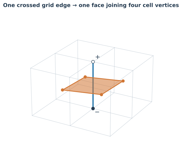
For our negative-inside convention, choose the winding so the face points toward the positive side. Use the same vertex index wherever a cell participates in a face. If a renderer needs triangles, a quad \((v_0,v_1,v_2,v_3)\) can be split into \((v_0,v_1,v_2)\) and \((v_0,v_2,v_3)\). For nonplanar quads, the chosen diagonal affects the displayed geometry.
The complete uniform-grid pipeline is therefore:
for each grid edge with opposite endpoint signs:
    compute and cache its intersection and normal

for each cell incident to a crossed edge:
    collect its cached Hermite samples
    fit one dual vertex

for each crossed interior grid edge:
    gather incident cells in cyclic order
    emit a segment in 2D or an oriented quad in 3D
A surface that reaches the sampling box needs an explicit boundary policy. The examples below instead use a box large enough to contain the whole surface.
A Complete Circle Example
Take
on the grid whose coordinates are \(-3,-2,\ldots,3\). At an edge crossing \(\mathbf p\), the unit normal is \(\mathbf p/2.5\).
The grid contains \(6\times6\) cells. Only 20 are active. Solving their QEFs and connecting across crossed edges produces 20 vertices and 20 segments forming a single closed loop.
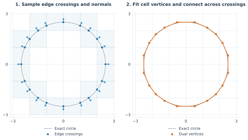
For example, in the cell \([1,2]\times[1,2]\), two crossings are \((1.5,2)\) and \((2,1.5)\). Their tangent lines are
Subtracting the equations gives \(x=y\), and hence
This point lies inside the cell but just outside the circle. It is exactly the intersection of the two tangent lines. That small example makes the QEF's objective concrete: agreement with tangent constraints does not mean projection onto the original surface.
From the Circle to a Sphere
Now use the same grid in three dimensions:
There are \(6^3=216\) cells. The implementation produces 128 vertices and 126 quads. The interactive display splits those quads into 252 triangles, while the dark lines show the original quad boundaries.
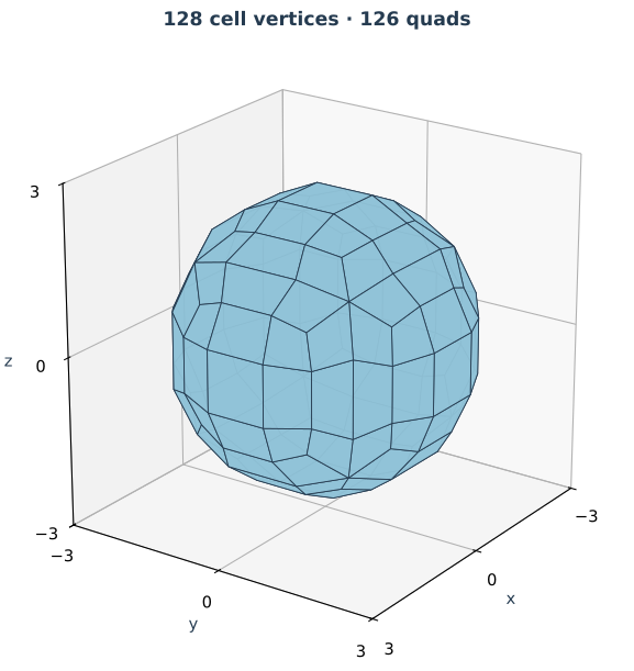
Drag to rotate the mesh. The legend lets you reveal the cell vertices and an exact reference sphere, or hide the surface to inspect its edges. You can also open the interactive figure separately.
For this mesh, every undirected edge belongs to exactly two faces, adjacent faces traverse a shared edge in opposite directions, and both display triangles of every quad face outward. It has 252 distinct quad edges, so
as expected for a sphere. These are useful checks on this example, not a proof that the same algorithm handles every sign configuration correctly.
Run the Examples
The contour implementation requires only NumPy. The figure generator additionally uses Matplotlib and Plotly. From the repository root, with those dependencies installed:
python content/code/2026-10-12-dual-contouring/dual_contouring.py
python content/code/2026-10-12-dual-contouring/make_figures.py
python content/code/2026-10-12-dual-contouring/test_dual_contouring.py
The first command prints the circle and sphere counts. The second regenerates the four SVG figures and the self-contained interactive HTML. The geometry checks cover the corner fit, a translated planar patch, the constrained minimization example, a connected circle loop, and sphere meshes at two resolutions.
This is deliberately a small uniform-grid implementation. It refines bracketed crossings by bisection, normalizes gradients, solves QEFs within cell bounds, and emits connectivity from cached crossed edges. It rejects exact grid-corner zeros and surfaces crossing the sampling-box boundary. It assumes at most one crossing per edge and does not resolve ambiguous topology or implement octree simplification.
What Changes on an Adaptive Octree?
Uniform grids spend the same resolution everywhere. An octree allows eight child cells to be represented by a larger parent where sufficient detail can be retained. In the original paper, adaptivity is a central part of the method, rather than a later add-on.
The QEFs can be combined:
A candidate parent vertex is evaluated against that combined error, together with topology checks before accepting a collapse. A small residual measures agreement with tangent planes; it is not by itself a bound on surface distance or a guarantee that a thin component survives.
At transitions between coarse and fine cells, connectivity must follow the octree's minimal edges, rather than treating each leaf independently as a uniform cube. A minimal edge is not subdivided by a neighboring leaf. Its incident leaf vertices form the corresponding polygon; transitions may produce triangles instead of quads. Ju and colleagues describe the recursive traversal in Section 3 of the original paper.
Crack-Free Does Not Mean Manifold
Three properties should be kept separate:
- Crack-free connectivity: neighboring pieces share their boundaries, without accidental gaps at cell or resolution transitions.
- Manifold topology: each point has a neighborhood like a disk for a closed surface. In particular, each mesh edge belongs to two faces, and the faces around each vertex form a single fan.
- Geometric validity: the realized faces do not fold over or intersect in unwanted ways.
A mesh can have no boundary gaps and still contain a non-manifold edge or a pinched vertex. One vertex per cell is particularly restrictive when several disconnected surface pieces pass through the same cell. A four-crossing configuration in a 2D cell already shows why a single vertex may join branches that ought to remain separate.
Schaefer, Ju, and Warren's Manifold Dual Contouring addresses manifoldness during adaptive simplification through additional topology-aware machinery. That guarantee should not be attributed to the basic one-vertex-per-cell construction.
For practical use, accurate Hermite samples, a stable QEF solve, and correct connectivity are all necessary. Refinement or a topology-aware variant is needed when the cell representation cannot express the local surface. Adjusting vertex positions alone cannot recover components that sampling never detected.
What to Take from the Construction
Dual Contouring makes a useful division of work. The QEF asks where a vertex best agrees with local surface orientations. The signed grid asks which vertices belong to the same mesh element. At a sharp corner, independent tangent constraints meet at a precise location. On a flat patch, they leave freedom that must be resolved sensibly.
Keeping those two steps distinct makes both the mathematics and the implementation easier to reason about. If a corner is rounded off, inspect the Hermite data and the fit. If the mesh has extra connections or missing faces, inspect the crossed-edge traversal. If separate sheets have merged, examine whether one vertex per cell was sufficient to represent them in the first place.
References
- Tao Ju, Frank Losasso, Scott Schaefer, and Joe Warren, Dual Contouring of Hermite Data, SIGGRAPH 2002, ACM Transactions on Graphics 21(3), pp. 339–346.
- Scott Schaefer and Joe Warren, Dual Contouring: “The Secret Sauce”. Implementation details, QEF representations, and mass-point handling of rank-deficient fits.
- Scott Schaefer, Tao Ju, and Joe Warren, Manifold Dual Contouring, IEEE Transactions on Visualization and Computer Graphics 13(3), 2007, pp. 610–619.
- NumPy,
numpy.linalg.lstsq, for the least-squares solver used in the examples.
Comments