Imagine riding a bicycle through a shallow puddle and leaving two curved tire tracks behind you. Can we find the area between those tracks without knowing an equation for either one? Under the usual idealization that the wheels roll without slipping sideways, the bicycle itself gives us the geometry we need: a segment of constant length, joining the rear wheel to the front wheel, is always tangent to the rear wheel's path. This is one of the examples in Tom Apostol's A Visual Approach to Calculus Problems, and it is a lovely invitation to think about integration geometrically.

The idea behind it is Mamikon's theorem: move tangent segments so that they start at a common point, and the area they sweep remains the same. A curved strip can become a disk, and an area under an exponential can be related to a triangle. Let's see why this works and how far we can take it.

The Ring That Started It

Start with two concentric circles. A chord of the outer circle touches the inner circle, and its length is $2L$. What is the area of the ring between the circles?

If their radii are $r$ and $R$, the radius to the point of tangency is perpendicular to the chord. The resulting right triangle gives

$$ R^2=r^2+L^2. $$

Therefore the area of the ring is

$$ A=\pi(R^2-r^2)=\pi L^2. $$

The inner radius has disappeared. Every such ring has the same area as a disk of radius $L$, however large its hole becomes.

According to Apostol's account, this was the problem that prompted Mamikon Mnatsakanian's discovery in 1959, while he was an undergraduate at Yerevan University. He went on to work in astrophysics and published his geometric method in 1981. Apostol later helped explain and develop it through their work at Caltech and Project MATHEMATICS! The history and classroom demonstrations are described in Apostol's 2000 article, pp. 23–26.

Mamikon's question was more interesting than the calculation: can we see why the inner circle does not matter?

Take just half of the chord, from its point of tangency to the outer circle. It is a tangent segment of length $L$. As it travels once around the inner circle, it sweeps out the entire ring. Now translate each segment, keeping its length and direction, until all the points of tangency coincide. The segments become the radii of a disk.

Figure 1. Use the slider or Play button to add corresponding tangent segments. Here r = 2, L = 1.5, and R = 2.5, so both shaded regions have area 2.25π.

The animation samples 48 segments; the filled backgrounds show the complete regions swept by a continuously moving segment. A finite collection of line segments alone has zero area. You can also open the interactive figure separately.

Tangent Sweeps and Tangent Clusters

We need two names for this construction:

A tangent sweep is the region traced by a segment that stays tangent to a curve at one endpoint. Its length may vary as it moves.
A tangent cluster is formed by translating those segments parallel to themselves until their points of tangency coincide.

Mamikon's theorem states that the tangent sweep and its corresponding tangent cluster have equal areas. Apostol and Mnatsakanian give the statement and a differential-geometric proof in Subtangents—An Aid to Visual Calculus, Sections 1 and 5.

For ordinary areas of regions, we must check that each region is swept just once. If segments retrace or overlap a region, the theorem compares areas counted with multiplicity; an oriented version keeps track of signs. We will first use examples where the relevant pieces do not overlap.

Why should translation preserve the swept area? Think of a very short part of the motion. Movement along the tangent contributes no area to first order: the segment is sliding along its own line. The turning of the segment produces a thin, almost triangular piece. Bringing the tangent segments to a common point preserves that turning and their lengths, and hence preserves these small contributions to the area.

For a convex polygon this is especially easy to picture. A segment sliding along a straight side sweeps no area. At each vertex it turns through the exterior angle and sweeps a circular sector. The exterior angles add to $2\pi$, so the sectors assemble into one disk. Approximating a smooth convex curve by polygons suggests the same result for an oval.

Consequently, a constant tangent length $L$ gives area $\pi L^2$ around any smooth, closed convex curve, including an ellipse. The outer boundary is traced by the free end of the tangent segment; it is generally not another ellipse or a curve at constant perpendicular distance from the inner one.

For a partial sweep with constant length and a monotone change of tangent direction through an angle $\Delta\theta$, with $|\Delta\theta|\le2\pi$, the cluster is a circular sector:

$$ A=\frac12 L^2|\Delta\theta|, $$

with angles measured in radians. We will return to this formula when we get back on the bicycle.

There is also a useful variation: we can bring the other endpoints of the tangent segments together instead. The resulting cluster is a centrally reflected copy of the first, so its area is the same. This is the version we will use for curves whose tangent segments end on the horizontal axis.

Subtangents: A Geometric Way to Read a Derivative

For a graph $y=f(x)$, take the tangent at $P=(x,f(x))$, with $f(x)\ne0$, and let it meet the horizontal axis at $Q$. Write

$$ Q=(x-s(x),0). $$

The signed horizontal displacement $s(x)$ is the subtangent. Since the tangent's slope is its vertical rise divided by its horizontal run,

$$ f'(x)=\frac{f(x)}{s(x)}, \qquad s(x)=\frac{f(x)}{f'(x)}, $$

where $f'(x)\ne0$. The subtangent is a projection of the tangent segment, not the segment's full length.

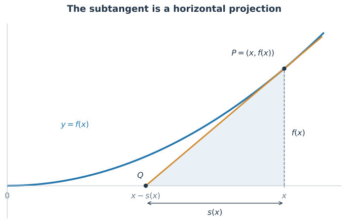
A point P on a curve, its tangent meeting the horizontal axis at Q, and a right triangle with height f(x) and signed horizontal base s(x). — Figure 2. Knowing the subtangent locates a second point on the tangent line.

The construction is simple: drop a perpendicular from $P$ to the horizontal axis, move horizontally by $-s(x)$, and join the resulting point to $P$. For some familiar functions, this becomes particularly convenient:

Curve	Subtangent $s(x)$	Horizontal intercept of the tangent
$y=e^{x/b}$, $b\ne0$	$b$	$x-b$
$y=x^n$, $x>0$, $n\ne0$	$x/n$	$x-x/n$
$y=1/x$, $x>0$	$-x$	$2x$

These examples come from Apostol and Mnatsakanian, Sections 2–3. Notice that a negative subtangent places the intercept to the right of the point's vertical projection. Also, multiplying $f$ by a nonzero constant does not change $s$, because the same factor appears in $f'$.

This gives a geometric characterization of exponentials. If the subtangent is a nonzero constant $b$, then $f'=f/b$, whose nonzero solutions are $f(x)=Ce^{x/b}$. We can recognize the whole family by the same little horizontal distance appearing in every tangent triangle.

The Area Under an Exponential

Let

$$ y=e^{x/b},\qquad b>0, $$

and choose a right endpoint $x=a$. Write $Y=e^{a/b}$. We want the area $A$ under the curve from $-\infty$ to $a$.

Every tangent segment from $(t,e^{t/b})$ to the horizontal axis ends at $(t-b,0)$. Move each of these intercepts to the origin. Its other endpoint becomes

$$ (b,e^{t/b}). $$

As $t$ runs from $-\infty$ to $a$, the translated endpoints run up the vertical line at horizontal coordinate $b$, from height approaching zero to height $Y$. Their segments fill a right triangle of base $b$ and height $Y$.

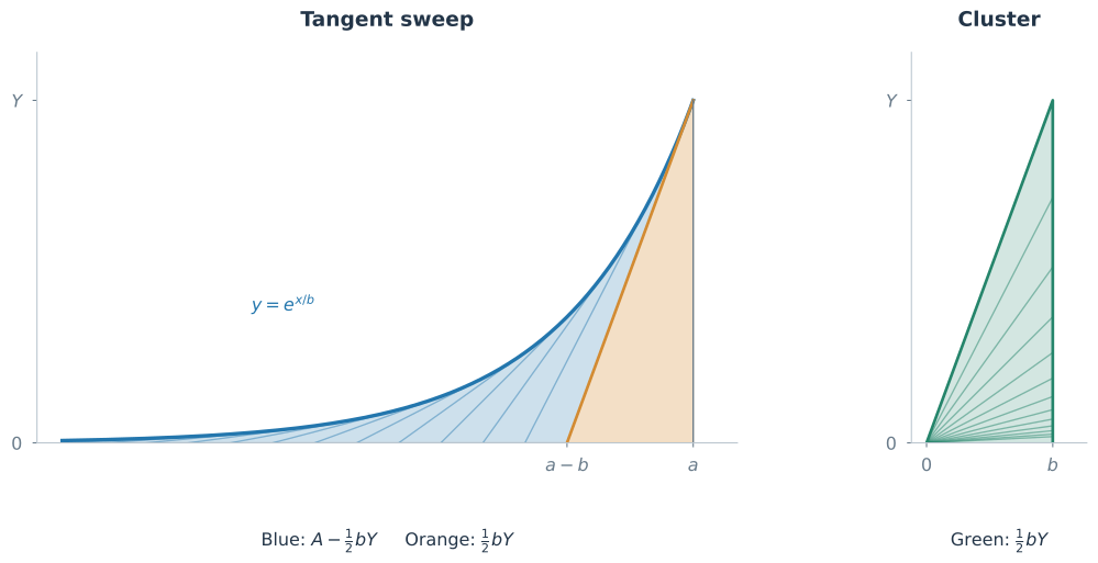
Left: the area under an exponential divided into a blue tangent sweep and an orange terminal triangle. Right: the translated tangent segments fill a triangle of base b and height Y. — Figure 3. The blue sweep has the same area as the green cluster. The orange triangle is the remaining part of the area under the curve.

Here is the detail that makes the argument work: the tangent sweep is not the entire area under the exponential. It leaves out the triangle below the final tangent, with vertices $(a-b,0)$, $(a,0)$, and $(a,Y)$. That triangle also has base $b$ and height $Y$.

Mamikon's theorem therefore gives

$$ A-\frac12 bY=\frac12 bY, $$

and so

$$ \boxed{A=bY=be^{a/b}.} $$

The full area is twice the area of either triangle. This is the construction in Apostol's article, p. 27. In the diagram the far-left tail is cut off for display; the argument uses the limit as the endpoint moves to $-\infty$.

Integration confirms the same result:

$$ \int_{-\infty}^{a}e^{x/b}\,dx=be^{a/b}. $$

The geometric argument makes the factor $b$ visible as a horizontal length.

The Parabola and Higher Powers

Next consider $y=x^2$ between $0$ and $a$, where $a>0$. Let its area be $A$ and write $Y=a^2$.

The subtangent at $(t,t^2)$ is $t/2$, so its tangent meets the axis at $(t/2,0)$. Translating that intercept to the origin sends the point on the parabola to

$$ \left(\frac{t}{2},t^2\right). $$

If we call the new horizontal coordinate $q$, these endpoints lie on $y=(2q)^2$: a horizontally compressed copy of the original parabola.

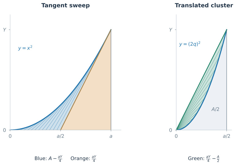
Left: the area under a parabola separated into its tangent sweep and the triangle below the final tangent. Right: the cluster lies between a straight line from the origin and a horizontally compressed parabola. — Figure 4. The two tangent regions have equal area. Compressing the parabola horizontally by a factor of two halves the area beneath it.

The final tangent cuts off a triangle of base $a/2$ and height $Y$, hence area $aY/4$. The sweep has area

$$ S=A-\frac{aY}{4}. $$

On the cluster side, the straight segment from the origin to $(a/2,Y)$ bounds another triangle of area $aY/4$. Beneath the compressed parabola is an area $A/2$. The cluster is the difference:

$$ C=\frac{aY}{4}-\frac A2. $$

Equating $S$ and $C$ gives

$$ A-\frac{aY}{4}=\frac{aY}{4}-\frac A2, \qquad \boxed{A=\frac{aY}{3}=\frac{a^3}{3}.} $$

Thus the area under this part of the parabola is one-third of its enclosing rectangle. This is Apostol's parabola construction, expressed as an equality between the sweep and cluster areas. See pp. 28–29 of his article.

The same reasoning works for $y=x^n$ with $n>1$. Now $Y=a^n$, the subtangent is $x/n$, and the cluster endpoints lie on $y=(nq)^n$. Horizontal compression divides the area by $n$, while each terminal triangle has area $aY/(2n)$. Hence

$$ A-\frac{aY}{2n}=\frac{aY}{2n}-\frac An, $$

which yields

$$ \boxed{A=\frac{aY}{n+1}=\frac{a^{n+1}}{n+1}.} $$

The familiar denominator $n+1$ emerges from adding the original area to its compressed copy.

A Cycloid Arch Contains Three Disks' Worth of Area

A cycloid is the curve traced by a point on the rim of a circular disk rolling along a straight line without slipping. If the radius is $r$, one complete turn carries the disk a horizontal distance $2\pi r$, and the highest point of the arch is $2r$ above the line. The enclosing rectangle therefore has area

$$ (2\pi r)(2r)=4\pi r^2. $$

We will find the area above the cycloid, inside that rectangle, and subtract it.

Let $P$ be the tracing point, $B$ the disk's contact point with the ground, and $Q$ the top of the disk. At each instant the disk rotates about $B$, so the velocity of $P$ is perpendicular to $BP$. Since $BQ$ is a diameter, the inscribed angle $BPQ$ is a right angle. Thus $PQ$ is tangent to the cycloid.

As the disk rolls, $Q$ moves along the top edge of the rectangle. The segments $PQ$ sweep the region between that edge and the cycloid.

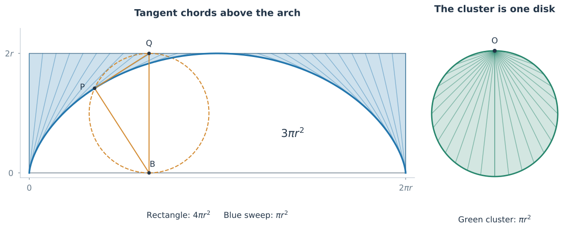
Left: a cycloid arch inside a rectangle, with tangent chords joining the curve to the top edge. Right: translating their upper endpoints to one point produces a disk of the same radius as the rolling disk. — Figure 5. The space above one cycloid arch has the area of one generating disk. The common endpoint O is on the boundary of the cluster disk, not at its center.

Now translate every $Q$ to a fixed point $O$ on that top line. This also brings all the rolling disks to the same position. The other endpoints, the translated copies of $P$, run around the circumference of that fixed disk. The tangent segments have become chords from $O$ that fill the disk: one half of the arch supplies one semicircle, and the other half supplies the other.

The cluster has area $\pi r^2$, so the region above the arch has that area too. Subtracting it from the rectangle gives

$$ \boxed{A_{\text{cycloid}}=4\pi r^2-\pi r^2=3\pi r^2.} $$

This argument appears in Apostol, p. 30, and in Peter Lynch's Mamikon's Visual Calculus and the Hodograph.

For comparison, the usual parametrization is

$$ x=r(\theta-\sin\theta),\qquad y=r(1-\cos\theta),\qquad 0\le\theta\le2\pi. $$

It leads to

$$ A=\int_0^{2\pi}r^2(1-\cos\theta)^2\,d\theta=3\pi r^2. $$

Both methods work. The geometric one explains the factor three through the decomposition of a rectangle into the arch area and a tangent sweep equal to one disk.

Back to the Bicycle: The Bicyclix and the Tractrix

Model the bicycle as a rigid segment of length $d$, its wheelbase, joining the two contact points with the ground. The rear wheel rolls in the direction of the frame, so that segment is tangent to the rear wheel's track. Its other endpoint traces the front wheel's track.

The region between the tracks, closed by the bicycle's initial and final positions, is a tangent sweep. If the frame turns monotonically through an angle $\Delta\theta$ and the sweep does not overlap itself, then

$$ \boxed{A=\frac12 d^2|\Delta\theta|.} $$

The angle here is the change in the frame's direction, not the steering angle of the front wheel relative to the frame. If the rear track is a simple closed convex curve and the bicycle makes one complete turn, the area between the tracks is $\pi d^2$.

For a winding ride that changes its turning direction, the contributions must be split into pieces. With a consistent orientation, the signed swept area is $d^2\Delta\theta/2$, using the accumulated, unwrapped change of direction. This may differ from the ordinary area of the visible union of the tracks. Lynch discusses such crossings in his bicycle example.

The tractrix is a special case: the front endpoint moves along a straight line while the rear endpoint follows it at a fixed distance. A toy pulled by a taut string gives the same construction. Starting with the string perpendicular to the line and pulling indefinitely, its direction approaches parallel to the line. The tangent cluster is a quarter-disk, so the area between this branch of the tractrix and its asymptote, closed by the initial string, is

$$ A=\frac12 d^2\frac\pi2=\frac{\pi d^2}{4}. $$

We did not need to solve for the tractrix's equation to find its area. The fixed string length and its quarter-turn were enough.

A Family Hidden Behind the Examples

The tractrix has a constant tangent length; the exponential has a constant subtangent. Apostol and Mnatsakanian connect these in Section 4 of their paper.

Let $\ell$ be the length of a tangent segment ending on a fixed baseline, and $s$ its nonnegative horizontal projection in the configuration under consideration. Suppose a curve satisfies

$$ \alpha\ell+\beta s=\gamma, $$

where $\alpha$ and $\beta$ are nonnegative and not both zero. Translating the baseline endpoints to the origin makes $\ell$ the distance from the origin to the cluster endpoint and $s$ its horizontal coordinate.

If $\beta=0$, the endpoints lie on a circle. If $\alpha=0$, they lie on a vertical line. If both coefficients are positive, rearranging gives

$$ \ell=\frac{\beta}{\alpha}\left(\frac{\gamma}{\beta}-s\right). $$

Put a vertical directrix at horizontal coordinate $\gamma/\beta$. The term in parentheses is the endpoint's distance to that line, while $\ell$ is its distance to the origin. This is precisely the focus–directrix definition of a conic, with eccentricity $\beta/\alpha$.

So the cluster boundary is part of an ellipse, parabola, or hyperbola according to that ratio. Constant tangents and constant subtangents are limiting cases of one geometric construction. Finding the original curve may require a differential equation, while recognizing its tangent cluster can be much easier.

Velocity Vectors and Hamilton's Hodograph

Lynch's article adds a connection to mechanics. A velocity vector is tangent to a body's trajectory. Translate all those velocity vectors to a common origin, and the curve traced by their tips is called a hodograph. The region swept by the arrows is the corresponding tangent cluster.

For an elliptic Kepler orbit under an inverse-square central force, Hamilton showed that the hodograph is a circle. The velocity changes both direction and magnitude, yet its tips trace this particularly simple curve. See Lynch's discussion and Figure 8.

There is a units issue to make explicit when interpreting this as an area in the orbital plane. A velocity is not a displacement. Choose a fixed time scale $\tau$ and draw tangent segments $\tau\mathbf v$ along the orbit. If the velocity-space hodograph has radius $V$, the scaled cluster has radius $\tau V$, and Mamikon's theorem gives the swept area, counted with multiplicity if needed, as

$$ A_{\text{sweep}}=\pi(\tau V)^2. $$

This is the area swept by those tangent segments; it is not the area enclosed by the elliptical orbit. The distinction matters because the cluster is built from velocity vectors, not position vectors.

Hodographs also appear in meteorology, where plotting wind vectors at different heights from a common origin makes changes in wind speed and direction visible. The shared idea is to remove the original locations of vectors so that their directions and lengths can be studied together.

Why the Theorem Works

The pictures suggest the theorem, but we can also check exactly which part of the motion contributes area. The following is a compact version of the differential-geometric argument in Apostol and Mnatsakanian, Section 5.

Let $\mathbf X(s)$ be a smooth curve parametrized by arc length, and let $\mathbf T(s)=\mathbf X'(s)$ be its unit tangent. Choose tangent segments of length $L(s)$. Their sweep is parametrized by

$$ \mathbf F(s,u)=\mathbf X(s)+u\mathbf T(s), \qquad 0\le u\le L(s). $$

The corresponding cluster, with its vertex at the origin, is

$$ \mathbf G(s,u)=u\mathbf T(s). $$

Their derivatives are

$$ \mathbf F_s=\mathbf T+u\mathbf T',\qquad \mathbf F_u=\mathbf T, $$

$$ \mathbf G_s=u\mathbf T',\qquad \mathbf G_u=\mathbf T. $$

Taking cross products, the extra translation term vanishes because $\mathbf T\times\mathbf T=0$:

$$ \mathbf F_s\times\mathbf F_u =u\mathbf T'\times\mathbf T =\mathbf G_s\times\mathbf G_u. $$

Both parametrizations therefore have the same local area element. Since $\mathbf T'$ is perpendicular to $\mathbf T$ and has magnitude equal to the curvature $\kappa(s)$,

$$ dA=u\kappa(s)\,du\,ds, $$

and integrating over the same parameter domain gives

$$ A_{\text{sweep}}=A_{\text{cluster}} =\frac12\int L(s)^2\kappa(s)\,ds. $$

For a plane curve, $\kappa(s)\,ds=|d\theta|$, so this becomes the familiar sector-area expression

$$ A=\frac12\int L(\theta)^2\,|d\theta|, $$

interpreted piece by piece when the tangent changes its direction of rotation. It also explains why overlapping sweeps require multiplicity accounting: these integrals measure the area of the parametrized sweep, including every pass.

The cross-product argument works for a space curve too. There the tangent sweep is a developable surface, and its translated cluster lies on a cone, possibly with singular points. Their surface areas agree; they need not lie in one plane.

What Visual Calculus Adds

The useful question to carry into another problem is: can I choose tangent segments whose translated endpoints form a simpler boundary? Constant length suggests a circle. Constant subtangent suggests a line. A rolling disk supplies tangent chords whose translated endpoints lie on another disk.

Recognizing that construction is the creative step. As Lynch observes, these methods do not offer the generality of ordinary calculus: a convenient geometric cluster is not always available. Even in our examples, derivatives helped us identify the subtangents, and a limiting argument underlies the smooth sweeps.

What the geometry offers is an explanation for the answer's shape. The exponential's area becomes two triangles. The power rule follows from horizontal compression. The cycloid's factor of three comes from removing one disk's worth of area from a rectangle containing four. Those are relationships we can see, and then return to when the formulas become too familiar to notice.

References and Figure Code

The three papers used here are:

Tom M. Apostol, A Visual Approach to Calculus Problems, Engineering & Science 63(3), 2000, pp. 22–31. The historical introduction and the annulus, exponential, parabola, bicycle, and cycloid constructions.
Tom M. Apostol and Mamikon A. Mnatsakanian, Subtangents—An Aid to Visual Calculus, The American Mathematical Monthly 109(6), 2002, pp. 525–533. Subtangents, the conic family, and the proof for tangent surfaces.
Peter Lynch, Mamikon's Visual Calculus and the Hodograph, Mathematics Today, April 2022. The supplied author's proof copy is numbered pp. 212–214. It discusses bicycle tracks, the cycloid, and Hamilton's hodograph.

Figures 2–5 were drawn for this post. The Python source uses NumPy and Matplotlib and writes the SVG figures to the matching image directory. From the repository root, with those packages installed, run:

python content/code/2026-10-09-visual-calculus/visual_calculus_figures.py

Comments

— comments

Curve	Subtangent \(s(x)\)	Horizontal intercept of the tangent
\(y=e^{x/b}\), \(b\ne0\)	\(b\)	\(x-b\)
\(y=x^n\), \(x>0\), \(n\ne0\)	\(x/n\)	\(x-x/n\)
\(y=1/x\), \(x>0\)	\(-x\)	\(2x\)

Visual Calculus